Realizing that I have not written anything here for two years lets just start writing again1: Compilation times for template-heavy C++ codebases such as the one at the center of my daily life can be a real pain. This mostly got worse since I started to really get my hands dirty in its depths during the extensive refactoring towards SIMD and GPU support2. The current sad high point in compilation times was reached when compiling the first GPU-enabled simulation cases: More than 100 seconds for a single compile on my not too shabby system. This article will detail how I significantly reduced this on the build system level while gaining useful features.
λ ~/p/c/o/e/t/nozzle3d (openlb-env-cuda-env) • time make make -C ../../.. core make[1]: Entering directory '/home/common/projects/contrib/openlb-master' make[1]: Nothing to be done for 'core'. make[1]: Leaving directory '/home/common/projects/contrib/openlb-master' nvcc -pthread --forward-unknown-to-host-compiler -x cu -O3 -std=c++17 --generate- code=arch=compute_75,code=[compute_75,sm_75] --extended-lambda --expt-relaxed- constexpr -rdc=true -DPLATFORM_CPU_SISD -DPLATFORM_GPU_CUDA - DDEFAULT_FLOATING_POINT_TYPE=float -I../../../src -c -o nozzle3d.o nozzle3d.cpp nvcc nozzle3d.o -o nozzle3d -lolbcore -lpthread -lz -ltinyxml -L/run/opengl- driver/lib -lcuda -lcudadevrt -lcudart -L../../../build/lib ________________________________________________________ Executed in 112.27 secs fish external usr time 109.46 secs 149.00 micros 109.46 secs sys time 2.42 secs 76.00 micros 2.42 secs
Even when considering that this compiles many dozens of individual CUDA kernels for multiple run-time selectable physical models and boundary conditions in addition to the simulation scaffold3 it still takes too long for comfortably iterating during development. Needless to say, things did not improve when I started working on heterogeneous execution and the single executable needed to also contain vectorized versions of all models for execution on CPUs in addition to MPI and OpenMP routines. Even worse, you really want to use Intel's C++ compilers when running CPU-based simulations on Intel-based clusters4 which plainly is not possible in such a homogeneous compiler setup where everyhing has to pass through nvcc
.
λ ~/p/c/o/e/t/nozzle3d (openlb-env-gcc-env) • time make g++ -O3 -Wall -march=native -mtune=native -std=c++17 -pthread - DPLATFORM_CPU_SISD -I../../../src -c -o nozzle3d.o nozzle3d.cpp g++ nozzle3d.o -o nozzle3d -lolbcore -lpthread -lz -ltinyxml -L../../.. /build/lib ________________________________________________________ Executed in 31.77 secs fish external usr time 31.21 secs 0.00 micros 31.21 secs sys time 0.55 secs 693.00 micros 0.55 secs
Comparing the GPU build to the previous CPU-only compilation time of around 32 seconds – while nothing to write home about – it was still clear that time would be best spent on separating out the CUDA side of things, both to mitigate its performance impact and to enabled a mixed compiler environment.
Firstly, any solution would need to exist within the existing plain Makefile based build system5 and should not complicate the existing build workflow for our users6. Secondly, it should allow for defining completely different compilers and configuration flags for the CPU- and the GPU-side of the application. The intial driving force of speeding up GPU-targeted compilation would then be satisfied as a side effect due to the ability of only recompiling the CPU-side of things as long as no new physical models are introduced. This restriction is useful in the present context as GPU kernels execute the computationally expensive part, i.e. the actual simulation, but generally do not change often during development of new simulation cases after the initial choice of physical model.
Following the requirements, a basic approach is to split the application into two compilation units: One containing only the CPU-implementation consisting of the high level algorithmic structure, pre- and post-processing, communication logic, CPU-targeted simulation kernels and calls to the GPU code. The other containing only the GPU code consisting of CUDA kernels and their immediate wrappers called from the CPU-side of things – i.e. only those parts that truly need to be compiled using NVIDIA's nvcc
. Given two separated files cpustuff.cpp
and gpustuff.cu
it would be easy to compile them using separate configurations and then link them together into a single executable. The main implementation problem is how to generate two such separated compilation units that can be cleanly linked together, i.e. without duplicating symbols and similar hurdles.
In days past the build system actually contained an option for such separated compilation: termed as the pre-compiled mode in OpenLB speak. This mode consisted of a somewhat rough and leaky separation between interface and implementation headers that was augmented by many hand-written C++ files containing explicit template instantiations of the aforementioned implementations for certain common arguments. These C++ files could then be compiled once into a shared library that was linked to the application unit compiled without access to the implementation headers. While this worked it was always a struggle to keep these files maintained. Additionally any benefit for the, at that time CPU-only, codebase was negligible and in the end not worth the effort any more causing it to be dropped somewhere on the road to release 1.4.
Nevertheless, the basic approach of compiling a shared libary of explicit template instantiations is sound if we can find a way to automatically generate the instantiations per-case instead of manually maintaining them. A starting point for this is to take a closer look at the linker errors produced when compiling a simulation case including only the interface headers for the GPU code. These errors contain partial signatures of all relevant methods from plain function calls
λ ~/p/c/o/e/l/cavity3dBenchmark (openlb-env-gcc-openmpi-cuda-env) • mpic++ cavity3d.o -lpthread -lz -ltinyxml -L../../../build/lib -lolbcore cavity3d.cpp:(...): undefined reference to `olb::gpu::cuda::device::synchronize() '
to bulk and boundary collision operator constructions
cavity3d.cpp:(...): undefined reference to `olb::ConcreteBlockCollisionO<float, olb::descriptors::D3Q19<>, (olb::Platform)2, olb::dynamics::Tuple<float, olb:: descriptors::D3Q19<>, olb::momenta::Tuple<olb::momenta::BulkDensity, olb:: momenta::BulkMomentum, olb::momenta::BulkStress, olb::momenta::DefineToNEq>, olb: :equilibria::SecondOrder, olb::collision::BGK, olb::dynamics::DefaultCombination> >::ConcreteBlockCollisionO()'
as well as core data structure accessors:
cavity3d.cpp:(.text. _ZN3olb20ConcreteBlockLatticeIfNS_11descriptors5D3Q19IJEEELNS_8PlatformE2EE21getP opulationPointersEj[ _ZN3olb20ConcreteBlockLatticeIfNS_11descriptors5D3Q19IJEEELNS_8PlatformE2EE21getP opulationPointersEj]+0x37): undefined reference to `olb::gpu::cuda::CyclicColumn< float>::operator[](unsigned long)'
These errors are easily turned into a sorted list of unique missing symbols using basic piping
build/missing.txt: $(OBJ_FILES) $(CXX) $^ $(LDFLAGS) -lolbcore 2>&1 \ | grep -oP ".*undefined reference to \`\K[^']+\)" \ | sort \ | uniq > $@
which only assumes that the locale is set to english and – surprisingly – works consistently accross any relevant C++ compilers7, likely due to all of them using either the GNU Linker or a drop-in compatible alternative thereto. The resulting plain list of C++ method signatures hints at the reasonably structured and consistent template language employed by OpenLB:
olb::ConcreteBlockCollisionO<float, olb::descriptors::D3Q19<>, (olb::Platform)2, olb::CombinedRLBdynamics<float, olb::descriptors::D3Q19<>, olb::dynamics::Tuple< float, olb::descriptors::D3Q19<>, olb::momenta::Tuple<olb::momenta::BulkDensity, olb::momenta::BulkMomentum, olb::momenta::BulkStress, olb::momenta::DefineToNEq>, olb::equilibria::SecondOrder, olb::collision::BGK, olb::dynamics:: DefaultCombination>, olb::momenta::Tuple<olb::momenta::VelocityBoundaryDensity<0, -1>, olb::momenta::FixedVelocityMomentumGeneric, olb::momenta:: RegularizedBoundaryStress<0, -1>, olb::momenta::DefineSeparately> > >:: ConcreteBlockCollisionO() olb::gpu::cuda::CyclicColumn<float>::operator[](unsigned long) olb::gpu::cuda::device::synchronize() // [...]
For example, local cell models – Dynamics in OpenLB speak – are mostly implemented as tuples of momenta, equilibrium functions and collision operators8. All such relevant classes tend to follow a consistent structure in what methods with which arguments and return types they implement. We can use this domain knowledge of our codebase to transform the incomplete signatures in our new missing.txt
into a full list of explicit template instantiations written in valid C++.
build/olbcuda.cu: build/missing.txt # Generate includes of the case source # (replaceable by '#include <olb.h>' if no custom operators are implemented in the application) echo -e '$(CPP_FILES:%=\n#include "../%")' > $@ # Transform missing symbols into explicit template instantiations by: # - filtering for a set of known and automatically instantiable methods # - excluding destructors # - dropping resulting empty lines # - adding the explicit instantiation prefix (all supported methods are void, luckily) cat build/missing.txt \ | grep '$(subst $() $(),\|,$(EXPLICIT_METHOD_INSTANTIATION))' \ | grep -wv '.*\~.*\|FieldTypeRegistry()' \ | xargs -0 -n1 | grep . \ | sed -e 's/.*/template void &;/' -e 's/void void/void/' >> $@ # - filtering for a set of known and automatically instantiable classes # - dropping method cruft and wrapping into explicit class instantiation # - removing duplicates cat build/missing.txt \ | grep '.*\($(subst $() $(),\|,$(EXPLICIT_CLASS_INSTANTIATION))\)<' \ | sed -e 's/\.*>::.*/>/' -e 's/.*/template class &;/' -e 's/class void/class/' \ | sort | uniq >> $@
Note that this is only possible due to full knowledge of and control over the target codebase. In case this is not clear already: In no way do I recommend that this approach be followed in a more general context9. It was only the quickest and most maintainable approach to achieving the stated requirements given the particulars of OpenLB.
As soon as the build system dumped the first olbcuda.cu
file into the build
directory I thought that all that remained was to compile this into a shared library and link it all together. However, the resulting shared library contained not only the explicitly instantiated symbols but also additional stuff that they required. This caused quite a few duplicate symbol errors when I tried to link the library and the main executable. While linking could still be forced by ignoring these errors, the resulting executable was not running properly. This is where I encountered something unfamiliar to me: linker version scripts.
The same as for basically every question one encounters in the context of such fundamental software as GNU ld
, first released alongside the other GNU Binutils in the 80s, a solution has long since been developed. For our particular problem the solution are linker version scripts.
LIBOLBCUDA { global: /* list of mangeled symbols to globally expose [...] */ _ZGVZN3olb9utilities14TypeIndexedMapIPNS_12AnyFieldTypeIfNS_11descriptors5D3Q19IJ EEELNS_8PlatformE0EEENS_17FieldTypeRegistryIfS5_LS6_0EEEE9get_indexINS_18Operator ParametersINS_19CombinedRLBdynamicsIfS5_NS_8dynamics5TupleIfS5_NS_7momenta5TupleI NSH_11BulkDensityENSH_12BulkMomentumENSH_10BulkStressENSH_11DefineToNEqEEENS_10eq uilibria11SecondOrderENS_9collision3BGKENSF_18DefaultCombinationEEENSI_INSH_18Inn erEdgeDensity3DILi0ELi1ELi1EEENSH_28FixedVelocityMomentumGenericENSH_17InnerEdgeS tress3DILi0ELi1ELi1EEENSH_16DefineSeparatelyEEEEEEEEEmvE5index; local: *; };
Such a file can be passed to the linker via the --version-script
argument and can be used to control which symbols the shared library should expose. For our mixed build mode the generation of this script is realized as an additional Makefile target:
build/olbcuda.version: $(CUDA_OBJ_FILES) echo 'LIBOLBCUDA { global: ' > $@ # Declare exposed explicitly instantiated symbols to prevent duplicate definitions by: # - filtering for the set of automatically instantiated classes # - excluding CPU_SISD symbols (we only instantiate GPU_CUDA-related symbols) # - dropping the shared library location information # - postfixing by semicolons nm $(CUDA_OBJ_FILES) \ | grep '$(subst $() $(),\|,$(EXPLICIT_CLASS_INSTANTIATION))\|cuda. *device\|checkPlatform' \ | grep -wv '.*sisd.*' \ | cut -c 20- \ | sed 's/$$/;/' >> $@ echo 'local: *; };' >> $@
Note that we do not need to manually mangle the symbols in our olbcuda.cu
but can simply read them from the library's object file using the nm
utility. The two instances of grep
are again the point where knowledge of the code base is inserted10.
At this point all that is left is to link it all together using some final build targets:
libolbcuda.so: $(CUDA_OBJ_FILES) build/olbcuda.version $(CUDA_CXX) $(CUDA_CXXFLAGS) -Xlinker --version-script=build/olbcuda.version -shared $(CUDA_OBJ_FILES) -o $@ $(EXAMPLE): $(OBJ_FILES) libolbcuda.so $(CXX) $(OBJ_FILES) -o $@ $(LDFLAGS) -L . -lolbcuda -lolbcore $(CUDA_LDFLAGS)
Here the shared library is compiled using the separately defined CUDA_CXX
compiler and associated flags while the example case is compiled using CXX
, realizing the required mixed compiler setup. For the final target we can now define a mode that only recompiles the main application while reusing the shared library:
$(EXAMPLE)-no-cuda-recompile: $(OBJ_FILES) $(CXX) $^ -o $(EXAMPLE) $(LDFLAGS) -L . -lolbcuda -lolbcore $(CUDA_LDFLAGS) .PHONY: no-cuda-recompile no-cuda-recompile: $(EXAMPLE)-no-cuda-recompile
While the initial compile of both the main CPU application and the GPU shared library any additional recompile using make no-cuda-recompile
is sped up significantly. For example the following full compilation of a heterogeneous application with MPI, OpenMP, AVX-512 Vectorization on CPU and CUDA on GPU takes around 115 seconds:
λ ~/p/c/o/e/t/nozzle3d (openlb-env-gcc-openmpi-cuda-env) • time make mpic++ -O3 -Wall -march=native -mtune=native -std=c++17 -pthread - DPARALLEL_MODE_MPI -DPLATFORM_CPU_SISD -DPLATFORM_GPU_CUDA - DDEFAULT_FLOATING_POINT_TYPE=float -I../../../src -c -o nozzle3d.o nozzle3d.cpp mpic++ nozzle3d.o -lpthread -lz -ltinyxml -L../../../build/lib -lolbcore 2>&1 | grep -oP ".*undefined reference to \`\K[^']+\)" | sort | uniq > build/missing. txt nvcc -O3 -std=c++17 --generate-code=arch=compute_75,code=[compute_75,sm_75] -- extended-lambda --expt-relaxed-constexpr -rdc=true -I../../../src - DPARALLEL_MODE_MPI -DPLATFORM_CPU_SISD -DPLATFORM_GPU_CUDA -Xcompiler -fPIC -c - o build/olbcuda.o build/olbcuda.cu nvcc -O3 -std=c++17 --generate-code=arch=compute_75,code=[compute_75,sm_75] -- extended-lambda --expt-relaxed-constexpr -rdc=true -Xlinker --version- script=build/olbcuda.version -shared build/olbcuda.o -o libolbcuda.so mpic++ nozzle3d.o -o nozzle3d -lpthread -lz -ltinyxml -L../../../build/lib -L . -lolbcuda -lolbcore -L/run/opengl-driver/lib -lcuda -lcudadevrt -lcudart ________________________________________________________ Executed in 115.34 secs fish external usr time 112.68 secs 370.00 micros 112.68 secs sys time 2.68 secs 120.00 micros 2.68 secs
Meanwhile any additional compilation without introduction of new physical models (leading to the instantiation of additional GPU kernels) using make no-cuda-recompile
takes just 37 seconds:
λ ~/p/c/o/e/t/nozzle3d (openlb-env-gcc-openmpi-cuda-env) • time make no-cuda- recompile mpic++ -O3 -Wall -march=native -mtune=native -std=c++17 -pthread - DPARALLEL_MODE_MPI -DPLATFORM_CPU_SISD -DPLATFORM_GPU_CUDA - DDEFAULT_FLOATING_POINT_TYPE=float -I../../../src -c -o nozzle3d.o nozzle3d.cpp mpic++ nozzle3d.o -o nozzle3d -lpthread -lz -ltinyxml -L../../../build/lib -L . -lolbcuda -lolbcore -L/run/opengl-driver/lib -lcuda -lcudadevrt -lcudart ________________________________________________________ Executed in 36.47 secs fish external usr time 35.71 secs 0.00 micros 35.71 secs sys time 0.75 secs 564.00 micros 0.75 secs
This speedup of ~3 for most compiles during iterative development alone is worth the effort of introducing this new mode. Additionally, the logs also already showcase mixed compilation as the CPU side of things is compiled using mpic++
resp. GNU C++ while the shared libary is compiled using nvcc
. This extends seamlessly to more complex setups combining MPI, OpenMP, AVX-512 vectorization on CPU and CUDA on GPU in a single application.
All in all this approach turned out to be unexpectedly stable and portable accross systems and compilers from laptops to supercomputers. While it certainly is not the most beautiful thing I ever implemented, to say the least, it is very workable in practice and noticeably eases day to day development. In any case, the mixed compilation mode was included in OpenLB release 1.6 and has worked without a hitch since then. The mixed compilation mode is also isolated to just a few optional Makefile targets and did not require any changes to the actual codebase – meaning that it can just quietly be dropped should a better solution for the requirements come along.
For the potentially empty set of people that have read this far, are interested in CFD simulations using LBM and did not run screaming from the rather pragmatic build solution presented here: If you want to spend a week learning about LBM theory and OpenLB practice from invited lecturers at the top of the field as well as my colleagues and me, our upcoming Spring School may be of interest. Having taken place for quite a few years now at diverse locations such as Berlin, Tunisia, Krakow and Greenwich the 2024 rendition will take place at the historical Heidelberger Akademie der Wissenschaften in March. I'd be happy to meet you there!
…and do my part in feeding the LLM training machine :-)↩︎
Definitely a double edged sword: On the one side it enables concise DSL-like compositions of physical models while supporting automatic code optimization and efficient execution accross heterogeneous hardware. On the other side my much younger, Pascal-fluent, self would not be happy with how cryptic and unmaintainable many of my listings can look to the outsider. In any case, OpenLB as a heavily templatized and meta-programmed C++ software library is a foundational design decision.↩︎
Data structures, pre- and post-processing logic, IO routines, …↩︎
Commonly improving performance by quite a few percent↩︎
Which was a deliberate design decision in order to minimize dependencies considering the minimal build complexity required by OpenLB as a plain CPU-only MPI code. While this could of course be reconsidered in the face of increased target complexity it was not the time to open that bottle.↩︎
Mostly domain experts from process engineering, physics or mathematics without much experience in software engineering.↩︎
Which spans various versions of GCC, Clang, Intel C++ and NVIDIA nvcc
↩︎
Momenta representing how to compute macroscopic quantities such as density and velocity, equilibrium representing the undistrubed representation of said quantities in terms of population values and the collision operator representing the specific function used to relax the current population towards this equilibrium. For more details on LBM see e.g. my articles on Fun with Compute Shaders and Fluid Dynamics, a Year of LBM or even my just-in-time visualized literate implementation.↩︎
However, implementing such a explicit instantiation generator that works for any C++ project could be an interesting project for… somebody.↩︎
Now that I write about it this could probably be modified to automatically and eliminate conflicts by only exposing the symbols that are missing from the main application↩︎
So for a change of scenery I recently started to mess around with microcontrollers again. Since the last time that I had any real contact with this area was probably around a decade ago — programming an ASURO robot — I started basically from scratch. Driven by the goal of building and programming a fancy mechanical keyboard (as it seems to be the trendy thing to do) I chose the Arduino-compatible Teensy 4.0 board. While I appreciate the rich and accessible software ecosystem for this platform, I don't really want to use some special IDE, applying amongst other things1 weird non-standard preprocessing to my code. In this vein it would also be nice to use my accustomed Nix-based toolchain which leads me to this article.
Roughly following what others did for Teensy 3.1 while adapting it to Teensy 4.0 and Nix flakes it is simple to build and flash some basic C++ programs onto a USB-attached board. The adapted version of the Arduino library is available on Github and can be compiled into a shared library using flags
MCU = IMXRT1062 MCU_DEF = ARDUINO_TEENSY40 OPTIONS = -DF_CPU=600000000 -DUSB_SERIAL -DLAYOUT_US_ENGLISH OPTIONS += -D__$(MCU)__ -DARDUINO=10813 -DTEENSYDUINO=154 -D$(MCU_DEF) CPU_OPTIONS = -mcpu=cortex-m7 -mfloat-abi=hard -mfpu=fpv5-d16 -mthumb CPPFLAGS = -Wall -g -O2 $(CPU_OPTIONS) -MMD $(OPTIONS) -ffunction-sections - fdata-sections CXXFLAGS = -felide-constructors -fno-exceptions -fpermissive -fno-rtti -Wno- error=narrowing -I@TEENSY_INCLUDE@
included into a run-of-the-mill Makefile and relying on the arm-none-eabi-gcc
compiler. Correspondingly, the derivation for the core library core.nix
is straight forward. It clones a given version of the library repository, jumps to the teensy4
directory, deletes the example main.cpp
file to exclude it from the library and applies a Makefile adapted from the default one. For the result only headers, common flags and the linker script IMXRT1062.ld
are exported.
As existing Arduino sketches commonly consist of a single C++ file (ignoring some non-standard stuff for later) most builds can be handled generically by a mapping of *.cpp
files into flashable *.hex
files. This is realized by the following function based on the teensy-core
derivation and a default makefile:
build = name: source: pkgs.stdenv.mkDerivation rec { inherit name; src = source; buildInputs = with pkgs; [ gcc-arm-embedded teensy-core ]; buildPhase = '' export CC=arm-none-eabi-gcc export CXX=arm-none-eabi-g++ export OBJCOPY=arm-none-eabi-objcopy export SIZE=arm-none-eabi-size cp ${./Makefile.default} Makefile export TEENSY_PATH=${teensy-core} make ''; installPhase = '' mkdir $out cp *.hex $out/ ''; };
The derivation yielded by build "test" ./test
results in a result
directory containing a *.hex
file for each C++ file contained in the test
directory. Adding a loader
function to be used in convenient nix flake run
commands
loader = name: path: pkgs.writeScript name '' #!/bin/sh ${pkgs.teensy-loader-cli}/bin/teensy-loader-cli --mcu=TEENSY40 -w ${path} '';
a reproducible build of the canonical blink example2 is realized using:
nix flake clone git+https://code.kummerlaender.eu/teensy-env --dest . nix run .#flash-blink
Expanding on this, the teensy-env
flake also provides convenient image(With)
functions for building programs that depend on additional Arduino libraries such as for controlling servos. E.g. the build of a program test.cpp
placed in a src
folder
#include <Arduino.h> #include <Servo.h> extern "C" int main(void) { Servo servo; // Servo connected to PWM-capable pin 1 servo.attach(1); while (true) { // Match potentiometer connected to analog pin 7 servo.write(map(analogRead(7), 0, 1023, 0, 180)); delay(20); } }
is fully described by the flake:
{ description = "Servo Test"; inputs = { teensy-env.url = git+https://code.kummerlaender.eu/teensy-env; }; outputs = { self, teensy-env }: let image = teensy-env.custom.imageWith (with teensy-env.custom.teensy-extras; [ servo ]); in { defaultPackage.x86_64-linux = image.build "servotest" ./src; }; }
At first I expected the build of uLisp3 to proceed equally smoothly as this implementation of Lisp for microcontrollers is provided as a single ulisp-arm.ino
file. However, the *.ino
extension is not just for show here as beyond even the replacement of main
by loop
and setup
— which would be easy to fix — it relies on further non-standard preprocessing offered by the Arduino toolchain. I quickly aborted my efforts towards patching in e.g. the forward-declarations which are automagically added during the build (is it really such a hurdle to at least declare stuff before referring to it… oh well) and instead followed a less pure approach using arduino-cli
to access the actual Arduino preprocessor.
arduino-cli core install arduino:samd arduino-cli compile --fqbn arduino:samd:arduino_zero_native --preprocess ulisp- arm.ino > ulisp-arm.cpp
The problematic line w.r.t. to reproducible builds in Nix is the installation of the arduino:samd
toolchain which requires network access and wants to install stuff to home. Pulling in arbitrary stuff over the network is of course not something one wants to do in an isolated and hopefully reproducible build environment which is why this kind of stuff is heavily restricted in common Nix derivations. Luckily it is possible to misuse (?) a fixed-output derivation to describe the preprocessing of ulisp-arm.ino
into a standard C++ ulisp-arm.cpp
compilable using the GCC toolchain.
The relevant file ulisp.nix
pulls in the uLisp source from Github and calls arduino-cli
to install its toolchain to a temporary home folder followed by preprocessing the source into the derivation's output. The relevant lines for turning this into a fixed-output derivation are
outputHashMode = "flat"; outputHashAlgo = "sha256"; outputHash = "mutVLBFSpTXgUzu594zZ3akR/Z7e9n5SytU6WoQ6rKA=";
to declare the hash of the resulting file. After this point building and flashing uLisp using the teensy-env
flake works the same as for any C++ program. The two additional SPI and Wire library dependencies are added easily using imageWith
:
teensy-ulisp = let ulisp-source = import ./ulisp.nix { inherit pkgs; }; ulisp-deps = with teensy-extras; [ spi wire ]; in (imageWith ulisp-deps).build "teensy-ulisp" (pkgs.linkFarmFromDrvs "ulisp" [ ulisp-source ]);
So we are now able to build and flash uLisp onto a conveniently attached Teensy 4.0 board using only:
nix flake clone git+https://code.kummerlaender.eu/teensy-env --dest . nix run .#flash-ulisp
Connecting finally via serial terminal screen /dev/ttyACM0 9600
we end up in a LISP environment where we can play around with the microcontroller at our leisure without reflashing.
59999> (* 21 2) 42 59999> (defun blink (&optional x) (pinmode 13 t) (digitalwrite 13 x) (delay 1000) (blink (not x))) 59966> (blink)
As always, the code of everything discussed here is available via Git on code.kummerlaender.eu. While I only focused on Teensy 4.0 it should be easy to adapt to other versions by changing the compiler flags using PaulStoffregen/cores as a reference.
LiterateLB's volumetric visualization functionality relies on a simple ray marching implementation to sample both the 3D textures produced by the simulation side of things and the signed distance functions that describe the obstacle geometry. While this produces surprisingly nice looking results in many cases, some artifacts of the visualization algorithm are visible depending on the viewport and sample values. Extending the ray marching code to utilize a noise function is one possibility of mitigating such issues that I want to explore in this article.
While my original foray into just in time visualization of Lattice Boltzmann based simulations was only an aftertought to playing around with SymPy based code generation approaches I have since put some work into a more fully fledged code. The resulting LiterateLB code combines symbolic generation of optimized CUDA kernels and functionality for just in time fluid flow visualization into a single literate document.
For all fortunate users of the Nix package manager, tangling and building this from the Org document is as easy as executing the following commands on a CUDA-enabled NixOS host.
git clone https://code.kummerlaender.eu/LiterateLB nix-build ./result/bin/nozzle
The basic ingredient for producing volumetric images from CFD simulation data is to compute some scalar field of samples . Each sample can be assigned a color by some convenient color palette mapping scalar values to a tuple of red, green and blue components.
The task of producing an image then consists to sampling the color field along a ray assigned to a pixel by e.g. a simple pinhole camera projection. For this purpose a simple discrete approximation of the volume rendering equation with constant step size already produces suprisingly good pictures. Specifically
is the color along ray of length with local absorption values . This local absorption value may be chosen seperately of the sampling function adding an additional tweaking point.
The basic approach may also be extended arbitrarily, e.g. it is only the inclusion of a couple of phase functions away from being able recover the color produced by light travelling through the participating media that is our atmosphere.
There are many different possibilities for the choice of sampling function given the results of a fluid flow simulation. E.g. velocity and curl norms, the scalar product of ray direction and shear layer normals or vortex identifiers such as the Q criterion
that contrasts the local vorticity and strain rate norms. The strain rate tensor is easily recovered from the non-equilibrium populations of the simulation lattice — and is in fact already used for the turbulence model. Similarly, the vorticity can be computed from the velocity field using a finite difference stencil.
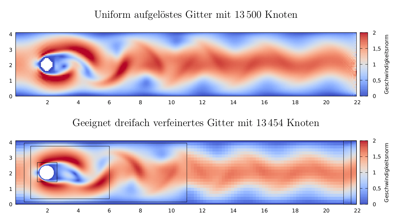
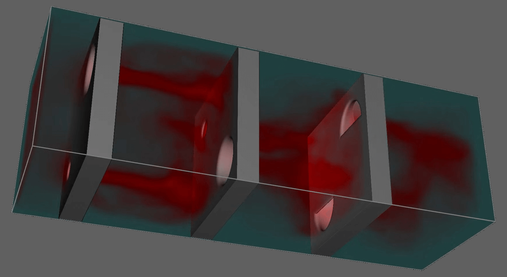
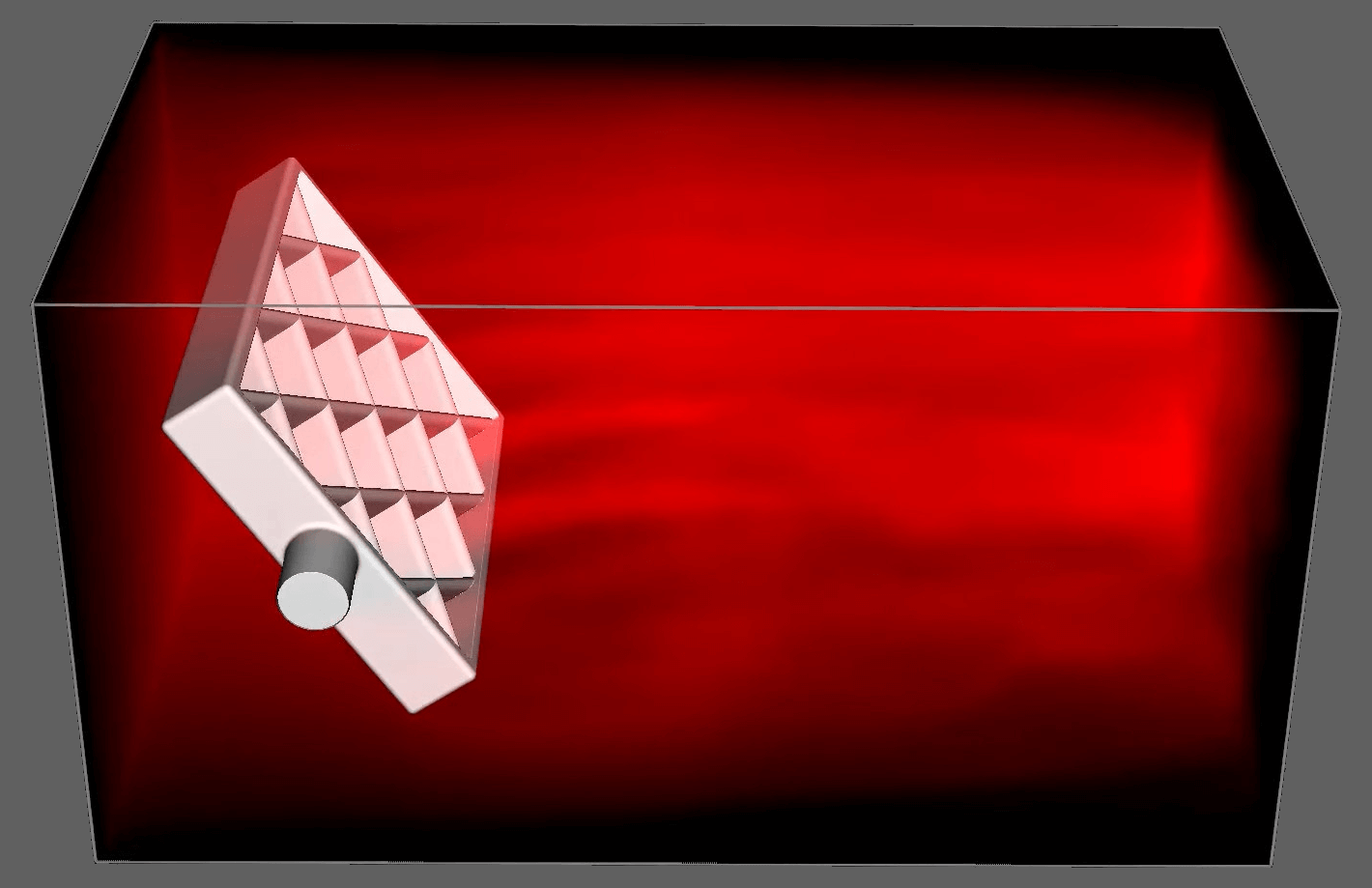
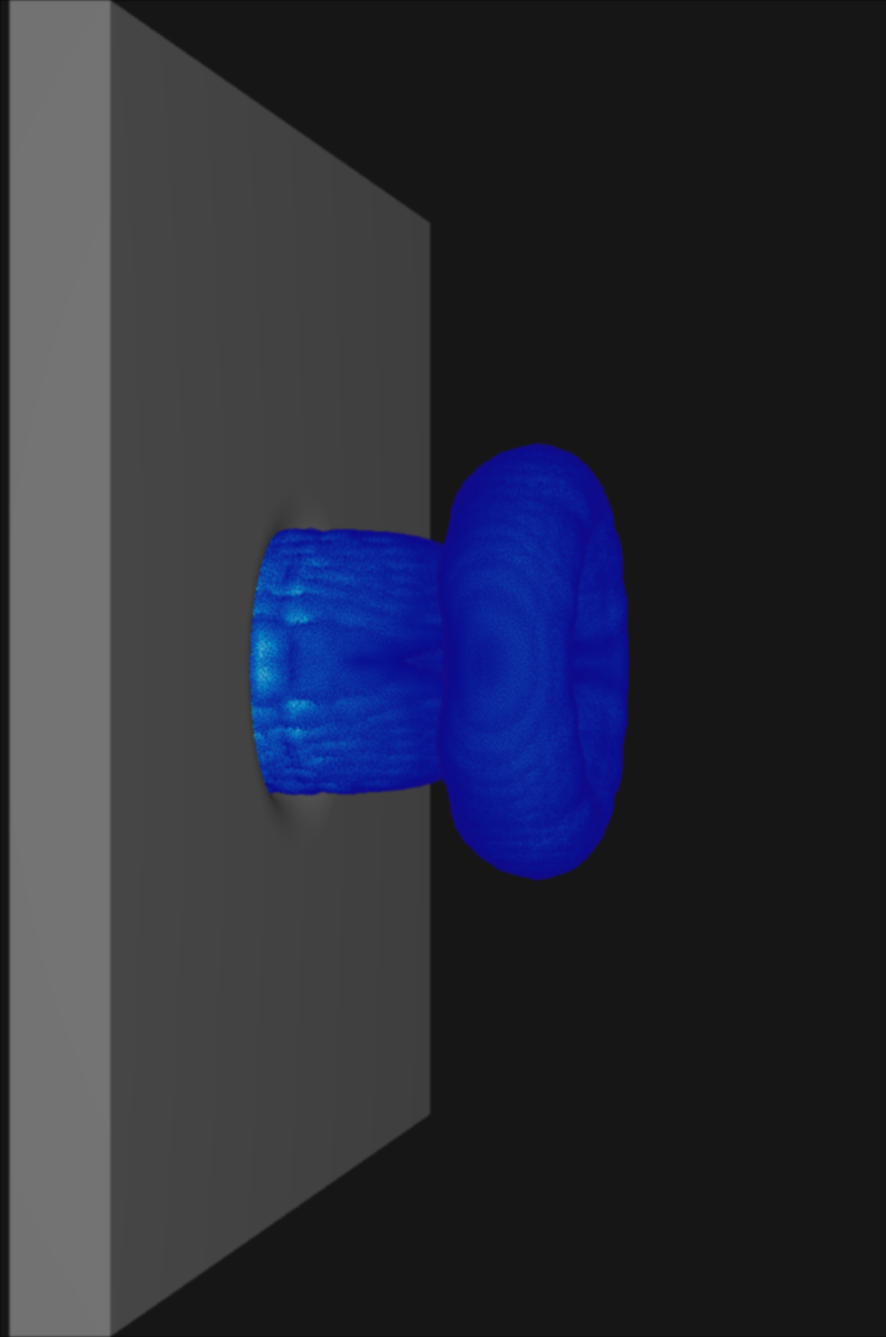
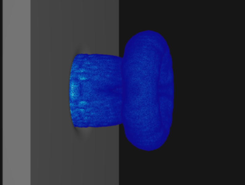
The problem w.r.t. rendering when thresholding sampling values to highlight structures in the flow becomes apparent in the following picture:
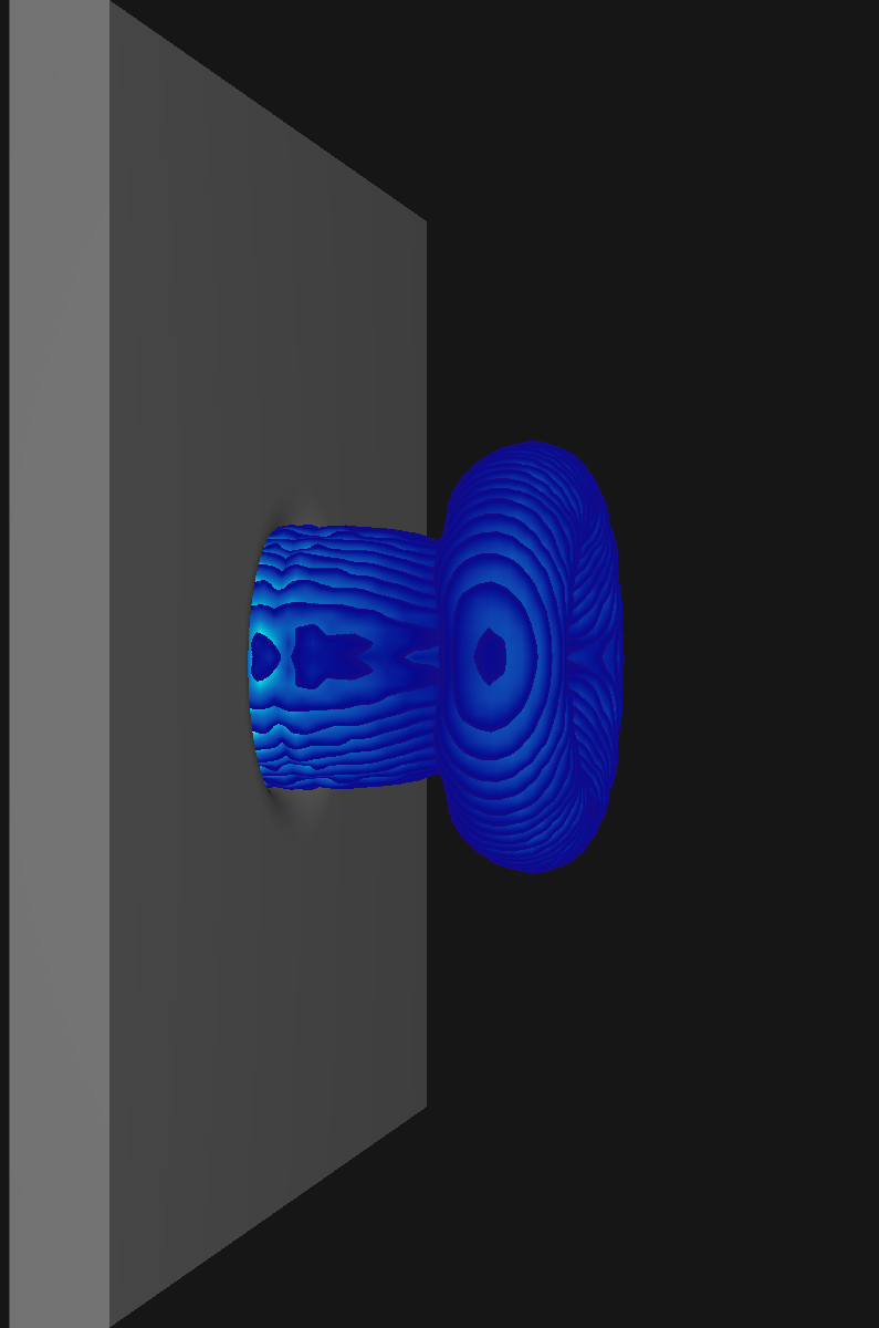
While the exact same volume discretization was used for both visualizations, the slices are much less apparent for the curl norm samples due to the more gradual changes. In general the issue is most prominent for scalar fields with large gradients (specifically the sudden jumps that occur when restricting sampling to certain value ranges as is the case for the Q criterion).
The reason for these artifacts is primarily choice of start offsets w.r.t. the traversed volume in addition the the step width. While this tends to become less noticable when decreasing said steps, this is not desirable from a performance perspective.
What I settled on for LiterateLB's renderer are view-aligned slicing and random jittering to remove most visible artifacts. The choice of randomness for jittering the ray origin is critical here as plain random numbers tend to produce a distracting static-like pattern. A common choice in practice is to use so called blue noise instead. While both kinds of noise eliminate most slicing artifacts, the remaining patterns tend to be less noticeable for blue noise. Noise is called blue if it contains only higher frequency components which makes it harder for the pattern recognizer that we call brain to find patterns where there should be none.
The void-and-cluster algorithm1 provides a straight forward method for pre-computing tileable blue noise textures that can be reused during the actual visualization. Tileability is a desirable property for this as we otherwise would either need a noise texture large enough to cover the entire image or instead observe jumps at the boundary between the tiled texture.
The first ingredient for void-and-cluster is a filteredPattern
function that applies a plain Gaussian filter with given to a cyclic 2d array. Using cyclic wrapping during the application of this filter is what renders the generated texture tileable.
def filteredPattern(pattern, sigma): return gaussian_filter(pattern.astype(float), sigma=sigma, mode='wrap', truncate=np.max(pattern.shape))
This function will be used to compute the locations of the largest void and tightest cluster in a binary pattern (i.e. a 2D array of 0s and 1s). In this context a void describes an area with only zeros and a cluster describes an area with only ones.
def largestVoidIndex(pattern, sigma): return np.argmin(masked_array(filteredPattern(pattern, sigma), mask=pattern))
These two functions work by considering the given binary pattern as a float array that is blurred by the Gaussian filter. The blurred pattern gives an implicit ordering of the voidness of each pixel, the minimum of which we can determine by a simple search. It is important to exclude the initial binary pattern here as void-and-cluster depends on finding the largest areas where no pixel is set.
def tightestClusterIndex(pattern, sigma): return np.argmax(masked_array(filteredPattern(pattern, sigma), mask=np. logical_not(pattern)))
Computing the tightest cluster works in the same way with the exception of searching the largest array element and masking by the inverted pattern.
def initialPattern(shape, n_start, sigma): initial_pattern = np.zeros(shape, dtype=np.bool) initial_pattern.flat[0:n_start] = True initial_pattern.flat = np.random.permutation(initial_pattern.flat) cluster_idx, void_idx = -2, -1 while cluster_idx != void_idx: cluster_idx = tightestClusterIndex(initial_pattern, sigma) initial_pattern.flat[cluster_idx] = False void_idx = largestVoidIndex(initial_pattern, sigma) initial_pattern.flat[void_idx] = True return initial_pattern
For the initial binary pattern we set n_start
random locations to one and then repeatedly break up the largest void by setting its center to one. This is also done for the tightest cluster by setting its center to zero. We do this until the locations of the tightest cluster and largest void overlap.
def blueNoise(shape, sigma):
The actual algorithm utilizes these three helper functions in four steps:
Initial pattern generation
n = np.prod(shape) n_start = int(n / 10) initial_pattern = initialPattern(shape, n_start, sigma) noise = np.zeros(shape)
Eliminiation of n_start
tightest clusters
pattern = np.copy(initial_pattern) for rank in range(n_start,-1,-1): cluster_idx = tightestClusterIndex(pattern, sigma) pattern.flat[cluster_idx] = False noise.flat[cluster_idx] = rank
Elimination of n/2-n_start
largest voids
pattern = np.copy(initial_pattern) for rank in range(n_start,int((n+1)/2)): void_idx = largestVoidIndex(pattern, sigma) pattern.flat[void_idx] = True noise.flat[void_idx] = rank
Elimination of n-n/2
tightest clusters of the inverted pattern
for rank in range(int((n+1)/2),n): cluster_idx = tightestClusterIndex(np.logical_not(pattern), sigma) pattern.flat[cluster_idx] = True noise.flat[cluster_idx] = rank
For each elimination the current rank
is stored in the noise texture producing a 2D arrangement of the integers from 0 to n
. As the last step the array is divided by n-1
to yield a grayscale texture with values in .
return noise / (n-1)
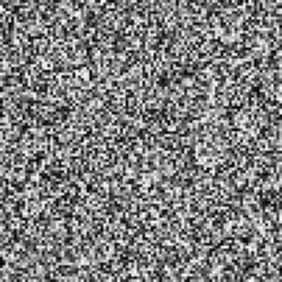
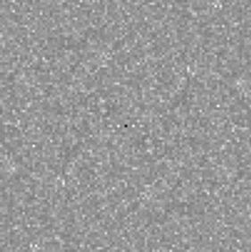
In order to check whether this actually generated blue noise, we can take a look at the Fourier transformation for an exemplary texture:
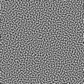
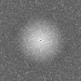
One can see qualitatively that higher frequency components are significantly more prominent than lower ones. Contrasting this to white noise generated using uniformly distributed random numbers, no preference for any range of frequencies can be observed:
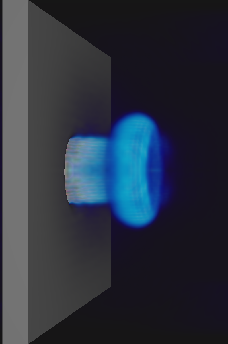
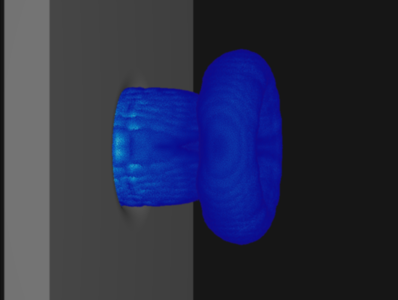
Contasting the original Q criterion visualization with one produced using blue noise jittering followed by a soft blurring shader, we can see that the slicing artifacts largely vanish. While the jittering is still visible to closer inspection, the result is significantly more pleasing to the eye and arguably more faithful to the underlying scalar field.
While white noise also obcures the slices, its lower frequency components produce more obvious static in the resulting image compared to blue noise. As both kinds of noise are precomputed we can freely choose the kind of noise that will produce the best results for our sampling data.
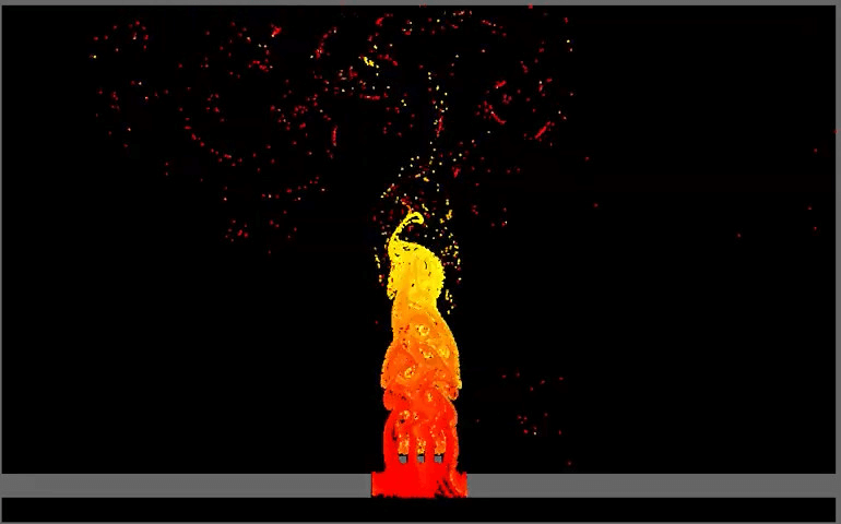
In practice where the noise is applied just-in-time during the visualization of a CFD simulation, all remaining artifacts tend to become invisible. This can be seen in the following video of the Q criterion evaluated for a simulated nozzle flow in LiterateLB:
Ulichney, R. Void-and-cluster method for dither array generation. In Electronic Imaging (1993). DOI: 10.1117/12.152707.↩︎
Suppose you have some kind of list of types. Such a list can by itself be used to perform any compile time computation one might come up with. So let us suppose that you additionally want to construct a tuple from something that is based on this list. i.e. you want to connect the compile time only type list to a run time object. In such a case you might run into new question such as: How do I call constructors for each of my tuple values? How do I offer access to the tuple values using only the type as a reference? How do I call a function for each value in the tuple while preserving the connection to the compile time list? If such questions are of interest to you, this article might possibly also be.
While the standard’s tuple template is part of the C++ subset I use in basically all of my developments1 I recently had to revisit some of these questions while reworking OpenLB’s core data structure using its meta descriptor concept. The starting point for this was a class template called FieldArrayD
to store an array of instances of a single field in a SIMD vectorization friendly structure of arrays layout. As a LBM lattice in practice stores not just one such field type but multiple of them (all declared in the central descriptor structure) I then wanted a MultiFieldArrayD
class template that does just that. i.e. a simple wrapper that accepts a list of fields as a variadic template parameter pack and instantiates a FieldArrayD
for each of them. A sensible place for storing these instances is of course our trusty std::tuple
:
/// SoA storage for instances of a single FIELD template<typename T, typename DESCRIPTOR, typename FIELD> struct FieldArrayD : public ColumnVector<T,DESCRIPTOR::template size<FIELD>()> { FieldArrayD(std::size_t count): ColumnVector<T,DESCRIPTOR::template size<FIELD>()>(count) { } /* [...] */ }; template<typename T, typename DESCRIPTOR, typename... FIELDS> class MultiFieldArrayD { private: std::tuple<FieldArrayD<T,DESCRIPTOR,FIELDS>...> _data; /* [...] */
A constructor for such a MultiFieldArrayD
class should now pass the same count of elements to each element constructor of the _data
tuple. This is more difficult than simply forwarding an individual value to each element which could be done using a common perfect forwarding pattern. But after some playing around I came up with a constructor
MultiFieldArrayD(std::size_t count): _count(count), // Trickery to construct each member of _data with `count`. // Uses the comma operator in conjunction with type dropping. _data((utilities::meta::void_t<FIELDS>(), count)...) { } { }
that does what I want in much more compact fashion that I expected at the beginning. Lets unwrap this: utilities::meta::void_t
is a place holder implementation of C++17’s std::void_t
that I use until we upgrade our C++14 code base2 to something more recent. In this case this somewhat aids the exposition as we can easily take a look at its definition:
template <typename...> using void_t = void;
If we consider this template to be a function it simply swallows any arguments it is given and returns void
. What we want to achieve is to duplicate the count
parameter sizeof...(FIELDS)
times and pass this parameter pack to the tuple’s perfect forwarding constructor. Such a pack is easily generated using the variadic expansion operator ...
. Sadly for this to work we have to have some kind of type-level dependency on the types in our pack which we do not really have when duplicating the count value (ignoring the number of times we want to duplicate). One kind of crafty way of getting a dependency anyway is to use the not very well known comma operator.
The comma operator forms a binary expression a, b
that evaluates both a
and b
but returns only b
. i.e. the expression (void_t<FIELDS>(), count)
depends on the types in the list FIELDS
but swallows them without using them in favour of returning count
. All in all this means that (void_t<FIELDS>(), count)...
will evaluate to a list of sizeof...(FIELDS)
copies of count
that are then passed as arguments to the tuple constructor. Note that if the field types are constructible we can also write e.g. (FIELDS(), count)...
but this doesn’t work for my use case as I do not want my description-only field types to be runtime instantiable.
The next thing we might want to do after successfully constructing a MultiFieldArrayD
is to access an individual FieldArrayD
instance. If we know the index of the desired field in the variadic list this is easily done using a plain call to std::get
. In practice I find that fields.get<FORCE>()
both looks nicer than e.g. fields.get<1>()
and is also self documenting which is always desirable. To do this we use the implicit assumption that types are not duplicated in our list and provide a recursive constexpr function to calculate the index:
template < typename WANTED_FIELD, typename CURRENT_FIELD, typename... FIELDS, // WANTED_FIELD equals the head of our field list, terminate recursion std::enable_if_t<std::is_same<WANTED_FIELD,CURRENT_FIELD>::value, int> = 0 > constexpr unsigned getIndexInFieldList() { return 0; } template < typename WANTED_FIELD, typename CURRENT_FIELD, typename... FIELDS, // WANTED_FIELD doesn't equal the head of our field list std::enable_if_t<!std::is_same<WANTED_FIELD,CURRENT_FIELD>::value, int> = 0 > constexpr unsigned getIndexInFieldList() { // Break compilation when WANTED_FIELD is not provided by list of fields static_assert(sizeof...(FIELDS) > 0, "Field not found."); return 1 + getIndexInFieldList<WANTED_FIELD,FIELDS...>(); }
This could probably be written more compactly using e.g. a std::conditional_t
alias template but this way we get a sensible assertion error when the field is not available. Furthermore as this function is also required in other areas of the field concept3 the actual call in MultiFieldArrayD
reads rather well:
template <typename FIELD> FieldArrayD<T,DESCRIPTOR,FIELD>& get() { return std::get<descriptors::getIndexInFieldList<FIELD,FIELDS...>()>(_data); }
The concept of swallowing during variadic pack expansion can also be utilized to call a lambda expression for each value of the tuple. This is useful as a building block for writing e.g. intialization or data serialization code that commonly needs to iterate over all fields. For example consider an extract of a copy assignment operator for a facade class representing a single cell of a lattice:
template <typename T, typename DESCRIPTOR> Cell<T,DESCRIPTOR>& Cell<T,DESCRIPTOR>::operator=(ConstCell<T,DESCRIPTOR>& rhs) { /* [...] */ this->_staticFieldsD.forFieldsAt(this->_iCell, [&rhs](auto field, auto id) { field = rhs.getFieldPointer(id); }); /* [...] */
Or a code snippet to serialize all field data to a sequential buffer:
T* currData = data + DESCRIPTOR::template size<descriptors::POPULATION>(); this->_staticFieldsD.forFieldsAt(this->_iCell, [&currData](auto field, auto id) { for (unsigned iDim=0; iDim < decltype(field)::d; ++iDim) { *(currData++) = field[iDim]; } });
The common element of these examples is of course the call to forFieldsAt
which is a template method of MultiFieldArrayD
. As its structure suggests the generic lambda expression is called for each field instance that belongs to the index _iCell
. The field
argument is an instance of some structure that provides access to the correct row of the FieldArrayD
instance belonging to the current field and id
is an identifier that can be used to connect this back to the actual field type (as the field
argument is a generic vector type that only carries the size of the row and not the field name).
template <typename F> void forFieldsAt(std::size_t idx, F f) { utilities::meta::swallow( (f(get<FIELDS>().getFieldPointer(idx), utilities::meta::id<FIELDS>{}), 0)... ); }
As we can see the expectations towards such a forFieldsAt
function are surprisingly easy to fullfill by using the swallow pattern. The utilities::meta::swallow
function is needed here as variadic pack expansion in some sense needs a place to expand into. In our previous example this was the tuple constructor but as we do not need to construct something here, swallow
fills the same niche.
/// Function equivalent of void_t, swallows any argument template <typename... ARGS> void swallow(ARGS&&...) { }
A closer look at the expanded comma operator expression shows that the function argument f
is passed two arguments and the void result is dropped in favour of returning and subsequently swallowing zero. The first argument is the reference to the requested row of our SoA storage and the second argument is a helper class to work around the non-custructability of the field type in this specific situation. Note that invoking f
using different argument types for each field works due to C++14’s generic lambda expressions. Any auto
arguments are templatized in the generated function call operator of the lambda stub class.
template <typename TYPE> struct id { using type = TYPE; };
Using this identity wrapper struct enables us to employ C++’s template argument deduction rules to access the field type without knowing the corresponding template parameter name in our generic lambda.
template <typename T, typename DESCRIPTOR> template <typename FIELD_ID> VectorPtr<T,DESCRIPTOR::template size<typename FIELD_ID::type>()> Cell<T,DESCRIPTOR>::getFieldPointer(FIELD_ID id) { return getFieldPointer<typename FIELD_ID::type>(); }
In theory both field type and field value access could be combined in a single argument of the generic lambda expression passed to forFieldsAt
but this would require field-specific VectorPtr
instantiations in my specific situation.
All in all this article illustrates another step I took in my quest to generate efficient data structures for population and field data from a single high-level type description while preserving self-documentation and static handling of the memory layout without any need for the user to juggle around raw offsets. The specific swallow pattern used in this instance is something I feel will come in handy in even more situations in the future. It really is much more compact and readable than any equivalent implementation using e.g. indexing sequences would be.
Also not the first time on this blog, e.g. mapping arrays using tuples in 2014 or mapping binary structures as tuples in 2013.↩︎
Not done yet as we need to support various older compilers and HPC environments. e.g. Intel’s compiler tends to be problematic in this context but yields significant performance gains for large simulations.↩︎
See expressive meta templates for flexible handling of compile-time constants for further examples↩︎
To both not leave the 2010s behind with just one measly article in their last year and to showcase some of the stuff I am currently working on this article covers a bouquet of topics – spanning both math-heavy theory and practical software development as well as travels to new continents. As to retroactively befit the title this past year of mine was dominated by various topics in the field of Lattice Boltzmann Methods. CFD in general and LBM in particular have shaped to become the common denominator of my studies, my work and even my leisure time.
The year began with the successful conclusion of my undergraduate studies of Mathematics at KIT. My corresponding Bachelor thesis discusses Grid refined Lattice Boltzmann Methods in OpenLB, in particular the approach taken by Lagrava et al. in Advances in Multi-domain Lattice Boltzmann Grid Refinement. The goal of such developments is to port one of the advantages of more classical approaches to fluid dynamics, namely Finite Element or Finite Volume methods, into the world of LBM: The ability to straight forwardly fit the discretizing mesh to the problem at hand. This feature is intrinsic to FEM as all computations are mapped from a physically embedded mesh of e.g. triangles into reference elements. The embedded mesh may be easily adapted to e.g. be more fine grained at boundaries or in other areas where the modeled fluid structures are more involved.
Doing this for the regular grids employed by LB implementations is more difficult in the sense that there is no intrinsic way to convert between differently resolved grids. Even more so it is not desirable to remove too much of the lattice structure regularity as this is one of the main aspects supporting the performance advantage which in turn is one of the method’s main selling points. On the theoretic side the main question is how to convert the population values at the contact surface between two differently resolved grids. Coming from a high resolution grid one has to decide how to restrict the more detailed information into a lower resolution and coming from a low resolution grid one has to find a way to recover the missing information compared to the targeted higher resolution. These questions are reflected directly in Lagrava’s approach by distinguishing between a restriction and an interpolation of the population’s non-equilibrium part.
The practical impact of my work during this thesis on OpenLB is a prototype implementation of grid refinement in 2D. In due time this will be expanded into a universally usable implementation for both two and three spatial dimensions but adding support for GPU-based computations to OpenLB currently enjoys a higher priority – but more on that later.
As one of the seminars required for my Master degree I studied how symbolic optimization, specifically common subexpression elimination, can help to automatically generate high performing LB implementations. To fit the overarching goal of my work the chosen target architecture for this were GPGPUs such as Nvidia’s P100.
As is detailed in the corresponding report I was pleasantly surprised by the performance resulting from code generated by formulating the LB collision step in the SymPy CAS library and applying the offered CSE optimization.
CSE | D2Q9 | D3Q19 | D3Q27 | |||
---|---|---|---|---|---|---|
single | double | single | double | single | double | |
No | 96.1% | 75.7% | 73.2% | 55.9% | 63.0% | 51.3% |
Yes | 95.6% | 96.4% | 96.9% | 98.7% | 94.9% | 99.8% |
Just as an example the table above lists the achieved performance on a P100 compared to the theoretical maximum on this platform before and after eliminating common subexpressions. The newer the hardware I test this on is, the less hand-optimization of the kernel code seems to matter. This nicely mirrors the historic development of CPUs where the hardware got better and better at efficiently executing code that is not optimized for a specific target CPU.
One of my current main interests is to expand on these results to develop a general framework for automatic Lattice Boltzmann kernel generation. The boltzgen library marks my first steps in this direction and is also my first serious use case for the Python ecosystem. Whereas I was originally not very fond of Python as a language – the switch from Python 2 to 3 and the surrounding issues as well as the syntax shaped my opinions there – the development speed and ease of expression kind of won me over during the course of this year. If one is mainly plugging together existing frameworks and delegating work to the GPU the resulting code tends to be more pleasant than a comparable development in e.g. C++.
Most of my working hours as a student employee of KIT’s Lattice Boltzmann Research Group were spent on two far reaching new developments: Implementing a template based framework for managing the memory of the various data fields required for LBM simulations and rewriting the essential Cell data structure into a pure data view. Details of the former are available in my article on Expressive meta templates for flexible handling of compile-time constants. The latter project lays the groundwork for my implementation of the Shift-Swap-Streaming propagation pattern that will be included in the next OpenLB release. This switch from the old collision-centric propagation pattern detailed by Mattila et al. in An Efficient Swap Algorithm for the Lattice Boltzmann Method to a new GPU- and vectorization-friendly algorithm is an important milestone in our ongoing quest to implement GPU-support in OpenLB. SSS is a very nice reformulation of the established single-grid A-A pattern into a plain collision step followed by changes to memory pointers in a central control structure. This means that streaming of information between neighboring lattice cells is not performed by explicitly moving memory around but rather by cunningly swapping and shifting some pointers. As an illustration:
Further details of this approach developed by Mohrhard et al. – in the same research group that I am currently working in – are available in An Auto-Vectorization Friendly Parallel Lattice Boltzmann Streaming Scheme for Direct Addressing.
At the time that I am writing this article I’ve only been back in Germany for about two weeks as I had the great opportunity to spend three weeks in Brazil at the University of Rio Grande do Sul. There I amongst other things held a talk on the Efficient parallel implementation of Lattice Boltzmann Methods – of which the slides in the previous section are an extract – as part of a workshop jointly organized by LBRG and SBCB.
I very much enjoyed my time in Porto Alegre and had the chance to discover Brazil as a country that I’d really like to spend more time travelling in – just look at some of the views we had during a weekend trip to Torres…
…and the Itaimbezinho canyon near Cambara do Sul:
After I ended up with a quite well performing GPU LBM code as a result of my seminar talk on symbolic code optimization I chose to expend some effort into developing nice looking real-time visualizations. Some of them are collected in my YouTube channel as well as linked behind the images in this section.
The quest to visualize three dimensional fluid flow led me into the field of computer graphics, specifically ray marching and signed distance functions. The former is useful when one considers the velocity field resulting from a simulation as a participating media through which light is shining while the latter may be used for describing, displaying and even voxelizing obstacle geometries.
For now the sources for these and other simulations still reside in a playground repository but one of my goals for the upcoming year is to further develop my own LB code based on the framework described in a previous section of this article. As an addition I also prototyped SDF-based indicator functions for OpenLB during my stay in Brazil and some form of support for this will be included in the upcoming release. Constructive solid geometry based on such functions offer a very flexible and information-rich concept for constructing simulation models. e.g. outer normals for certain boundary conditions are easily extracted from such a description.
As an example consider the full code of the grid fin geometry visualized above:
float sdf(vec3 v) { v = rotate_z(translate(v, v3(center.x/2, center.y, center.z)), -0.6); const float width = 1; const float angle = 0.64; return add( sadd( sub( rounded(box(v, v3(5, 28, 38)), 1), rounded(box(v, v3(6, 26, 36)), 1) ), cylinder(translate(v, v3(0,0,-45)), 5, 12), 1 ), sintersect( box(v, v3(5, 28, 38)), add( add( box(rotate_x(v, angle), v3(10, width, 100)), box(rotate_x(v, -angle), v3(10, width, 100)) ), add( add( add( box(rotate_x(translate(v, v3(0,0,25)), angle), v3(10, width, 100)), box(rotate_x(translate(v, v3(0,0,25)), -angle), v3(10, width, 100)) ), add( box(rotate_x(translate(v, v3(0,0,-25)), angle), v3(10, width, 100)) , box(rotate_x(translate(v, v3(0,0,-25)), -angle), v3(10, width, 100) ) ) ), add( add( box(rotate_x(translate(v, v3(0,0,50)), angle), v3(10, width, 100)), box(rotate_x(translate(v, v3(0,0,50)), -angle), v3(10, width, 100)) ), add( box(rotate_x(translate(v, v3(0,0,-50)), angle), v3(10, width, 100)) , box(rotate_x(translate(v, v3(0,0,-50)), -angle), v3(10, width, 100) ) ) ) ) ), 2 ) ); }
This quickly thrown together prototype is already somewhat reminiscent of how geometries are descibed by CSG-based CAD software packages such as OpenSCAD. As I just started out working on this I expect lots of further fun with this – and everthing else detailed in this article – for the upcoming year.