» A Year of Lattice Boltzmann
» December 31, 2019 | development english math | Adrian Kummerländer
To both not leave the 2010s behind with just one measly article in their last year and to showcase some of the stuff I am currently working on this article covers a bouquet of topics – spanning both math-heavy theory and practical software development as well as travels to new continents. As to retroactively befit the title this past year of mine was dominated by various topics in the field of Lattice Boltzmann Methods. CFD in general and LBM in particular have shaped to become the common denominator of my studies, my work and even my leisure time.
Grid refinement
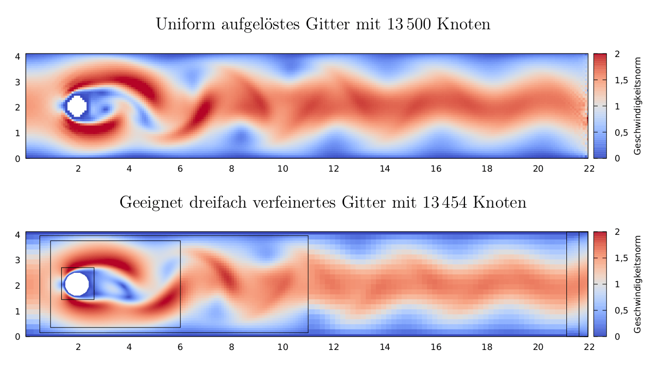
The year began with the successful conclusion of my undergraduate studies of Mathematics at KIT. My corresponding Bachelor thesis discusses Grid refined Lattice Boltzmann Methods in OpenLB, in particular the approach taken by Lagrava et al. in Advances in Multi-domain Lattice Boltzmann Grid Refinement. The goal of such developments is to port one of the advantages of more classical approaches to fluid dynamics, namely Finite Element or Finite Volume methods, into the world of LBM: The ability to straight forwardly fit the discretizing mesh to the problem at hand. This feature is intrinsic to FEM as all computations are mapped from a physically embedded mesh of e.g. triangles into reference elements. The embedded mesh may be easily adapted to e.g. be more fine grained at boundaries or in other areas where the modeled fluid structures are more involved.
Doing this for the regular grids employed by LB implementations is more difficult in the sense that there is no intrinsic way to convert between differently resolved grids. Even more so it is not desirable to remove too much of the lattice structure regularity as this is one of the main aspects supporting the performance advantage which in turn is one of the method’s main selling points. On the theoretic side the main question is how to convert the population values at the contact surface between two differently resolved grids. Coming from a high resolution grid one has to decide how to restrict the more detailed information into a lower resolution and coming from a low resolution grid one has to find a way to recover the missing information compared to the targeted higher resolution. These questions are reflected directly in Lagrava’s approach by distinguishing between a restriction and an interpolation of the population’s non-equilibrium part.
The practical impact of my work during this thesis on OpenLB is a prototype implementation of grid refinement in 2D. In due time this will be expanded into a universally usable implementation for both two and three spatial dimensions but adding support for GPU-based computations to OpenLB currently enjoys a higher priority – but more on that later.
Symbolic code generation
As one of the seminars required for my Master degree I studied how symbolic optimization, specifically common subexpression elimination, can help to automatically generate high performing LB implementations. To fit the overarching goal of my work the chosen target architecture for this were GPGPUs such as Nvidia’s P100.
As is detailed in the corresponding report I was pleasantly surprised by the performance resulting from code generated by formulating the LB collision step in the SymPy CAS library and applying the offered CSE optimization.
| CSE | D2Q9 | D3Q19 | D3Q27 | |||
|---|---|---|---|---|---|---|
| single | double | single | double | single | double | |
| No | 96.1% | 75.7% | 73.2% | 55.9% | 63.0% | 51.3% |
| Yes | 95.6% | 96.4% | 96.9% | 98.7% | 94.9% | 99.8% |
Just as an example the table above lists the achieved performance on a P100 compared to the theoretical maximum on this platform before and after eliminating common subexpressions. The newer the hardware I test this on is, the less hand-optimization of the kernel code seems to matter. This nicely mirrors the historic development of CPUs where the hardware got better and better at efficiently executing code that is not optimized for a specific target CPU.
One of my current main interests is to expand on these results to develop a general framework for automatic Lattice Boltzmann kernel generation. The boltzgen library marks my first steps in this direction and is also my first serious use case for the Python ecosystem. Whereas I was originally not very fond of Python as a language – the switch from Python 2 to 3 and the surrounding issues as well as the syntax shaped my opinions there – the development speed and ease of expression kind of won me over during the course of this year. If one is mainly plugging together existing frameworks and delegating work to the GPU the resulting code tends to be more pleasant than a comparable development in e.g. C++.
Meta templates and propagation patterns
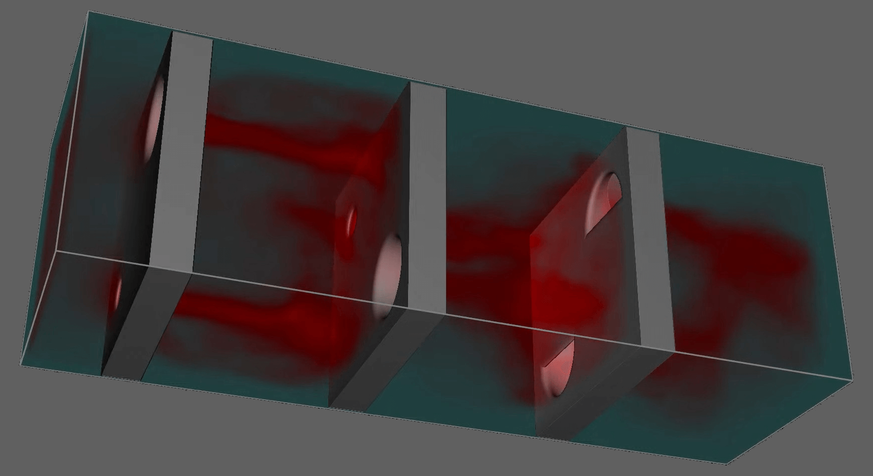
Most of my working hours as a student employee of KIT’s Lattice Boltzmann Research Group were spent on two far reaching new developments: Implementing a template based framework for managing the memory of the various data fields required for LBM simulations and rewriting the essential Cell data structure into a pure data view. Details of the former are available in my article on Expressive meta templates for flexible handling of compile-time constants. The latter project lays the groundwork for my implementation of the Shift-Swap-Streaming propagation pattern that will be included in the next OpenLB release. This switch from the old collision-centric propagation pattern detailed by Mattila et al. in An Efficient Swap Algorithm for the Lattice Boltzmann Method to a new GPU- and vectorization-friendly algorithm is an important milestone in our ongoing quest to implement GPU-support in OpenLB. SSS is a very nice reformulation of the established single-grid A-A pattern into a plain collision step followed by changes to memory pointers in a central control structure. This means that streaming of information between neighboring lattice cells is not performed by explicitly moving memory around but rather by cunningly swapping and shifting some pointers. As an illustration:
Further details of this approach developed by Mohrhard et al. – in the same research group that I am currently working in – are available in An Auto-Vectorization Friendly Parallel Lattice Boltzmann Streaming Scheme for Direct Addressing.
Brazil
At the time that I am writing this article I’ve only been back in Germany for about two weeks as I had the great opportunity to spend three weeks in Brazil at the University of Rio Grande do Sul. There I amongst other things held a talk on the Efficient parallel implementation of Lattice Boltzmann Methods – of which the slides in the previous section are an extract – as part of a workshop jointly organized by LBRG and SBCB.
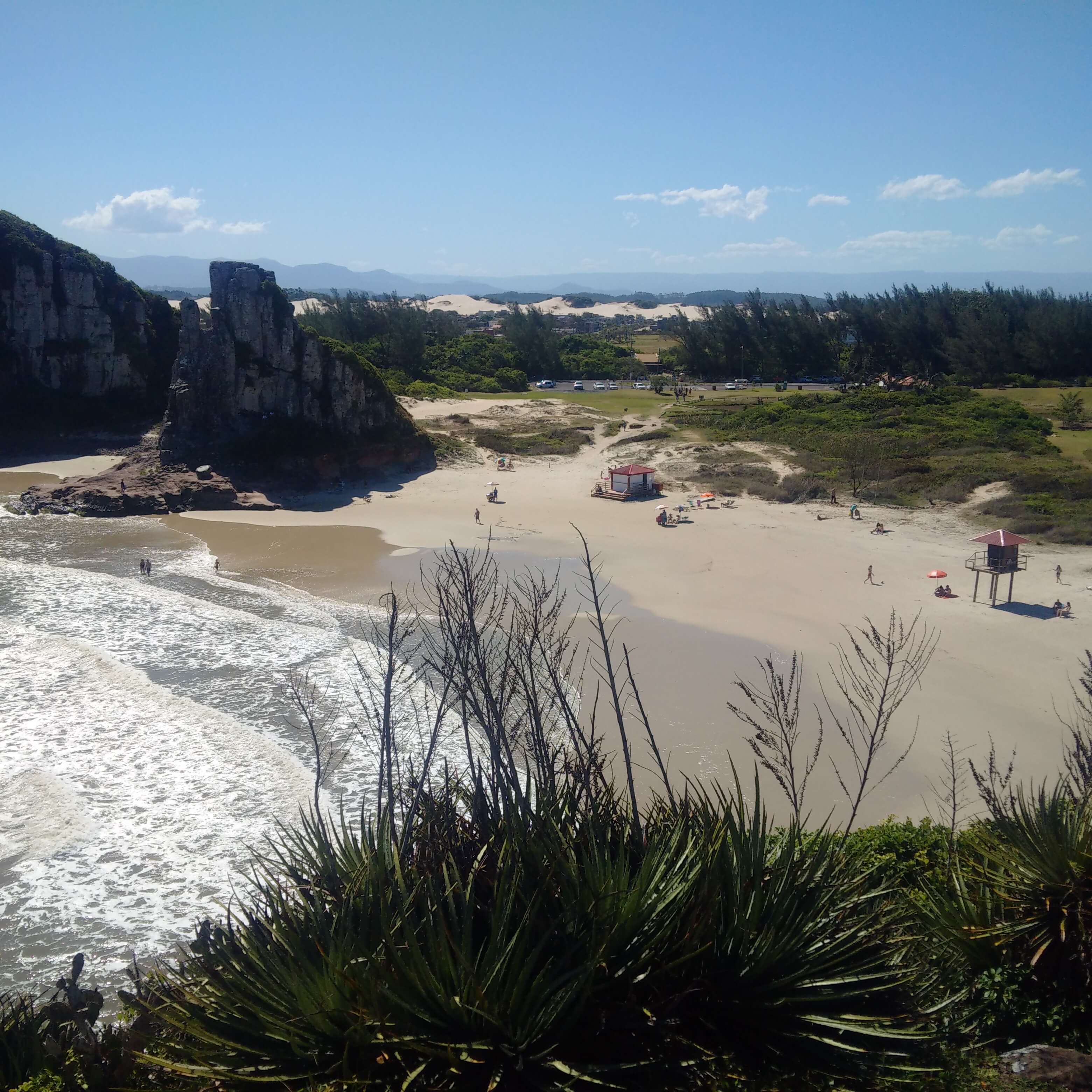
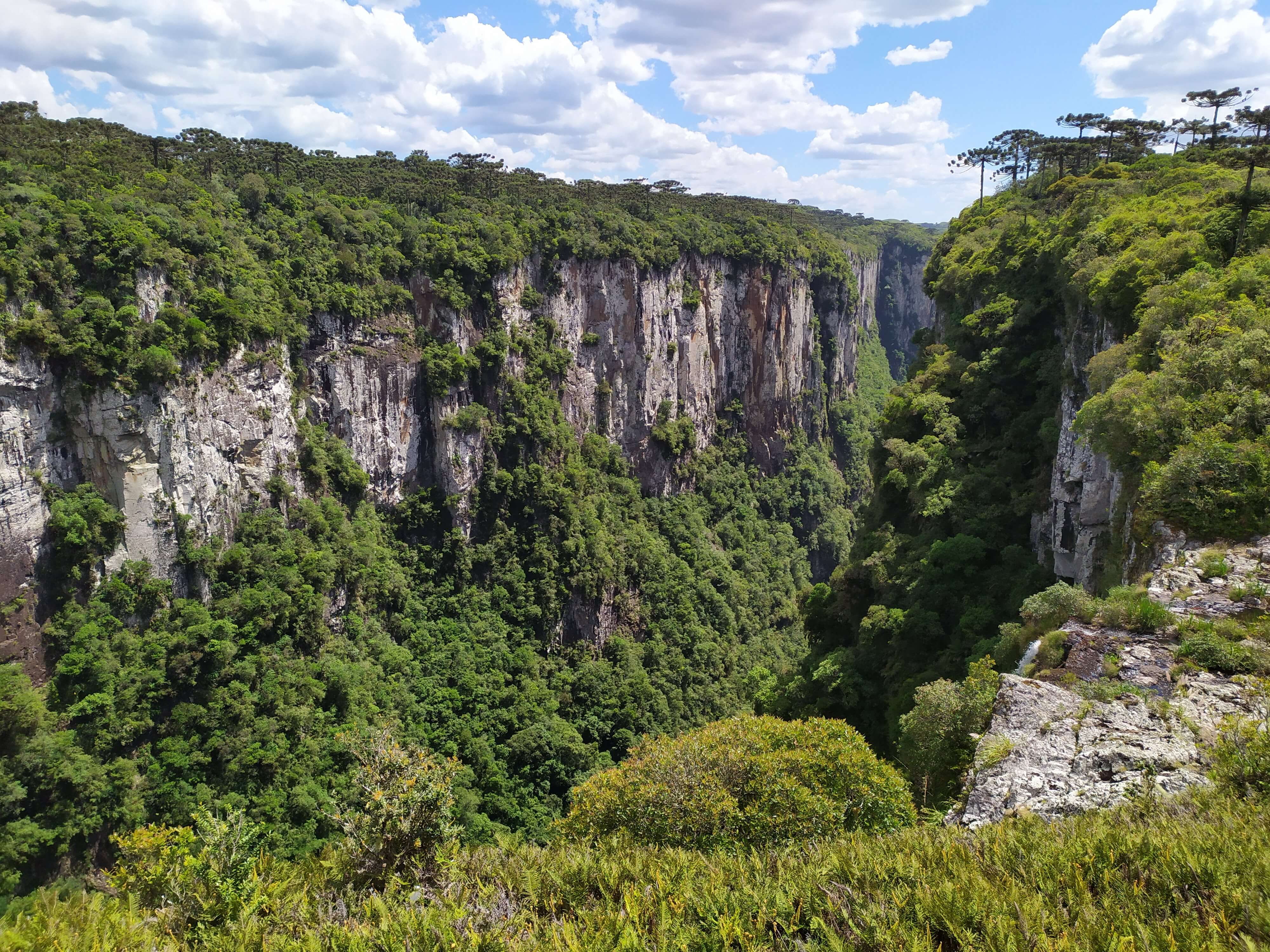
I very much enjoyed my time in Porto Alegre and had the chance to discover Brazil as a country that I’d really like to spend more time travelling in – just look at some of the views we had during a weekend trip to Torres…
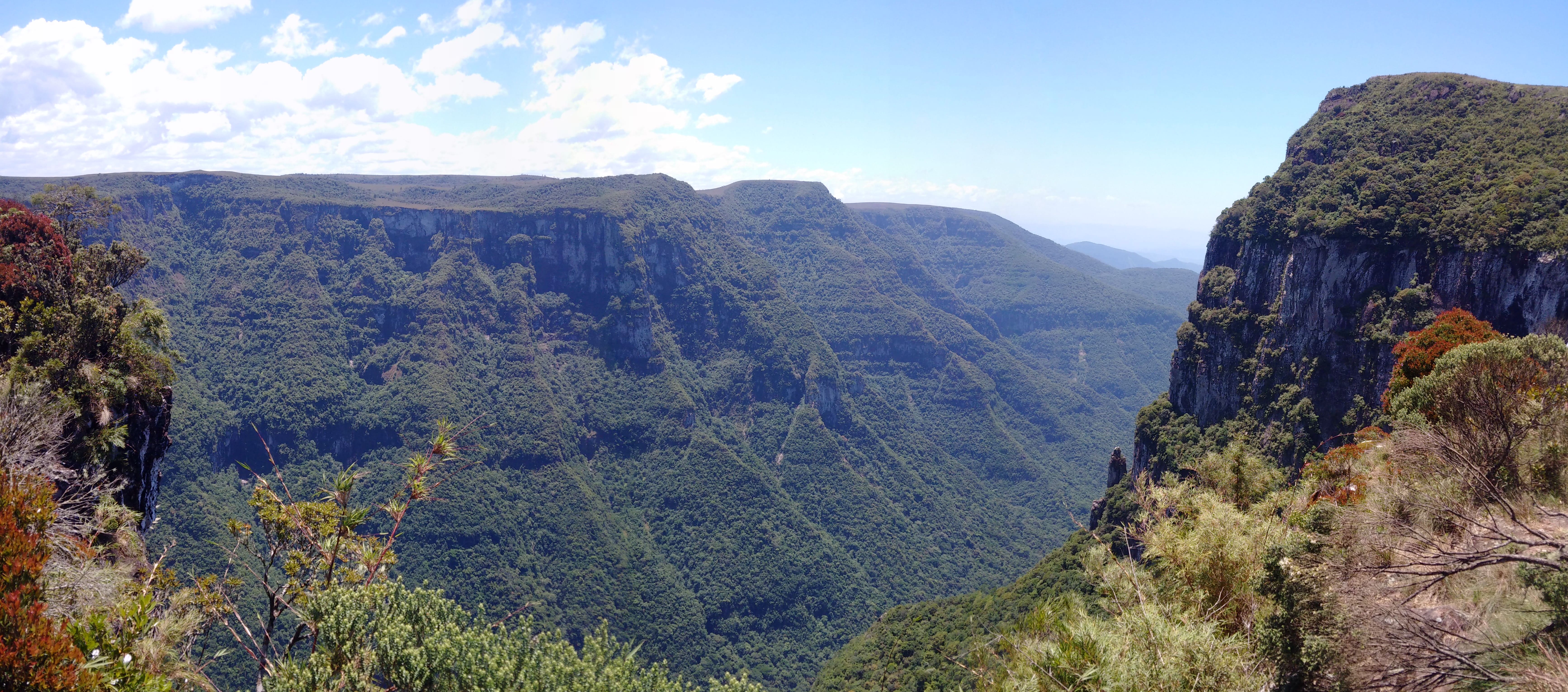
…and the Itaimbezinho canyon near Cambara do Sul:
The joy of signed distance functions
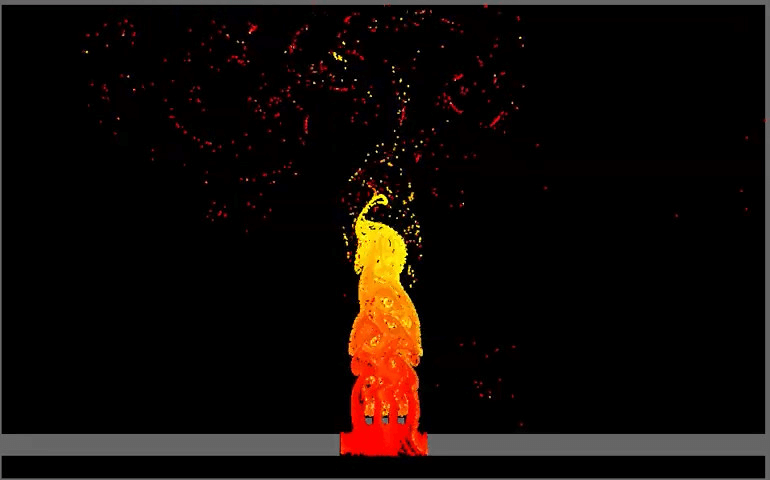
After I ended up with a quite well performing GPU LBM code as a result of my seminar talk on symbolic code optimization I chose to expend some effort into developing nice looking real-time visualizations. Some of them are collected in my YouTube channel as well as linked behind the images in this section.
The quest to visualize three dimensional fluid flow led me into the field of computer graphics, specifically ray marching and signed distance functions. The former is useful when one considers the velocity field resulting from a simulation as a participating media through which light is shining while the latter may be used for describing, displaying and even voxelizing obstacle geometries.
For now the sources for these and other simulations still reside in a playground repository but one of my goals for the upcoming year is to further develop my own LB code based on the framework described in a previous section of this article. As an addition I also prototyped SDF-based indicator functions for OpenLB during my stay in Brazil and some form of support for this will be included in the upcoming release. Constructive solid geometry based on such functions offer a very flexible and information-rich concept for constructing simulation models. e.g. outer normals for certain boundary conditions are easily extracted from such a description.
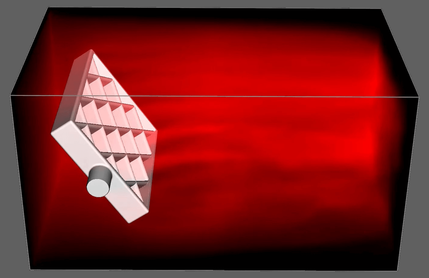
As an example consider the full code of the grid fin geometry visualized above:
float sdf(vec3 v) {
  v = rotate_z(translate(v, v3(center.x/2, center.y, center.z)), -0.6);
  const float width = 1;
  const float angle = 0.64;

  return add(
    sadd(
      sub(
        rounded(box(v, v3(5, 28, 38)), 1),
        rounded(box(v, v3(6, 26, 36)), 1)
      ),
      cylinder(translate(v, v3(0,0,-45)), 5, 12),
      1
    ),
    sintersect(
      box(v, v3(5, 28, 38)),
      add(
        add(
          box(rotate_x(v, angle), v3(10, width, 100)),
          box(rotate_x(v, -angle), v3(10, width, 100))
        ),
        add(
          add(
            add(
              box(rotate_x(translate(v, v3(0,0,25)), angle), v3(10, width, 100)),
              box(rotate_x(translate(v, v3(0,0,25)), -angle), v3(10, width, 100))
            ),
            add(
              box(rotate_x(translate(v, v3(0,0,-25)), angle), v3(10, width, 100))
              ,
              box(rotate_x(translate(v, v3(0,0,-25)), -angle), v3(10, width, 100)
              )
            )
          ),
          add(
            add(
              box(rotate_x(translate(v, v3(0,0,50)), angle), v3(10, width, 100)),
              box(rotate_x(translate(v, v3(0,0,50)), -angle), v3(10, width, 100))
            ),
            add(
              box(rotate_x(translate(v, v3(0,0,-50)), angle), v3(10, width, 100))
              ,
              box(rotate_x(translate(v, v3(0,0,-50)), -angle), v3(10, width, 100)
              )
            )
          )
        )
      ),
      2
    )
  );
}
This quickly thrown together prototype is already somewhat reminiscent of how geometries are descibed by CSG-based CAD software packages such as OpenSCAD. As I just started out working on this I expect lots of further fun with this – and everthing else detailed in this article – for the upcoming year.