/home/adrian

» Fun with compute shaders and fluid dynamics

» December 22, 2018 | cpp development english math | Adrian Kummerländer

As I previously alluded to, computational fluid dynamics is a current subject of interest of mine both academically¹ and recreationally². Where on the academic side the focus obviously lies on theoretical strictness and simulations are only useful as far as their error can be judged and bounded, I very much like to take a more hand wavy approach during my freetime and just fool around. This works together nicely with my interest in GPU based computation which is to be the topic of this article.

While visualizations such as the one above are nice to behold in a purely asthetic sense independent of any real word groundedness their implementation is at least inspired by models of our physical reality. The next section aims to give a overview of such models for fluid flows and at least sketch out the theoretical foundation of the specific model implemented on the GPU to generate all visualization we will see on this page.

Levels of abstraction

The behaviour of weakly compressible fluid flows – i.e. non-supersonic flows where the compressibility of the flowing fluid plays a small but non-central role – is commonly modelled by the weakly compressible Navier-Stokes equations which relate density $\rho$, pressure $p$, viscosity $\nu$ and speed $u$ to each other:

$\begin{aligned} \partial_t \rho + \nabla \cdot (\rho u) &= 0 \\ \partial_t u + (u \cdot \nabla) u &= -\frac{1}{\rho} \nabla p + 2\nu\nabla \cdot \left(\frac{1}{2} (\nabla u + (\nabla u)^\top)\right)\end{aligned}$

As such the Navier-Stokes equations model a continuous fluid from a macroscopic perspective. That means that this model doesn’t concern itself with the inner workings of the fluid – e.g. what it is actually made of, how the specific molecules making up the fluid interact individually and so on – but rather considers it as an abstract vector field. One other way to model fluid flows is to explicitly model the individual fluid molecules using classical physics. This microscopic approach closely reflects what actually happens in reality. From this perspective the flow of the fluid is just an emergent property of the underlying individual physical interactions. Which approach one chooses for computational fluid dynamics depends on the question one wants to answer as well as the available computational ressources. A sufficienctly precise model of individual molecular interactions precisely models physical reality in arbitrary situations but is easily much more computationally intensive that a macroscopic approach using Navier-Stokes. In turn, solving such macroscoping equations can quickly become problematic in complex geometries with diverse boundary conditions. No model is perfect and no model is strictly better that any other model in all categories.

Lattice Boltzmann in theory…

The approach I want to introduce for this article is neither macroscopic nor microscopic but situated between those two levels of abstraction – it is a mesoscopic approach to fluid dynamics. Such a model is given by the Boltzmann equations that can be used to describe fluids from a statistical perspective. As such the Boltzmann-approach is to model neither the macroscopic behavior of a fluid nor the microscopic particle interactions but the probability of a certain mass of fluid particles $f$ moving inside of an external force field $F$ with a certain directed speed $\xi$ at a certain spatial location $x$ at a specific time $t$:

$\left( \partial_t + \xi \cdot \partial_x + \frac{F}{\rho} \cdot \partial_\xi \right) f = \Omega(f) \left( = \partial_x f \cdot \frac{dx}{dt} + \partial_\xi f \cdot \frac{d\xi}{dt} + \partial_t f \right)$

The total differential $\Omega(f)$ of this Boltzmann advection equation can be viewed as a collision operator that describes the local redistribution of particle densities caused by said particles colliding. As this equation by itself is still continuous in all variables we need to discretize it in order to use it on a finite computer. This basically means that we restrict all variable values to a discrete and finite set in addition to replacing difficult to solve parts with more approachable approximations. Implementations of such a discretized Boltzmann equation are commonly referred to as the Lattice Boltzmann Method.

As our goal is to display simple fluid flows on a distinctly two dimensional screen, a first sensible restiction is to limit space to two dimensions³. As a side note: At first glance this might seem strange as no truly 2D fluids exist in our 3D environment. While this doesn’t need to concern us for generating entertaining visuals there are in fact some real world situations where 2D fluid models can be reasonable solutions for 3D problems.

The lattice in LBM hints at the further restriction of our 2D spatial coordinate $x$ to a discrete lattice of points. The canonical way to structure such a lattice is to use a cartesian grid.

Besides the spatial restriction to a two dimensional lattice a common step of discretizing the Boltzmann equation is to approximate the collision operator using an operator pioneered by Bhatnagar, Gross and Krook:

$\Omega(f) := -\frac{f-f^\text{eq}}{\tau}$

This honorifically named BGK operator relaxes the current particle distribution $f$ towards its theoretical equilibrium distribution $f^\text{eq}$ at a rate $\tau$. The value of $\tau$ is one of the main control points for influencing the behaviour of the simulated fluid. e.g. its Reynolds number⁴ and viscosity are controlled using this parameter. Combining this definition of $\Omega(f)$ and the Boltzmann equation without external forces yields the BGK approximation of said equation:

$(\partial_t + \xi \cdot \nabla_x) f = -\frac{1}{\tau} (f(x,\xi,t) - f^\text{eq}(x,\xi,t))$

To further discretize this we restrict the velocity $\xi$ not just to two dimensions but to a finite set of nine discrete unit velocities (D2Q9 - 2 dimensions, 9 directions):

$\newcommand{\V}[2]{\begin{pmatrix}#1\\#2\end{pmatrix}} \{\xi_i\}_{i=0}^8 = \left\{ \V{0}{0}, \V{-1}{\phantom{-}1}, \V{-1}{\phantom{-}0}, \V{-1}{-1}, \V{\phantom{-}0}{-1}, \V{\phantom{-}1}{-1}, \V{1}{0}, \V{1}{1}, \V{0}{1} \right\}$

We also define the equilibrium $f^\text{eq}$ towards which all distributions in this model strive as the discrete equilibrium distribution by Maxwell and Boltzmann. This distribution $f_i^\text{eq}$ of the $i$-th discrete velocity $\xi_i$ is given for density $\rho \in \mathbb{R}_{\geq 0}$ and total velocity $u \in \mathbb{R}^2$ as well as fixed lattice weights $w_i$ and lattice speed of sound $c_s$:

$f_i^\text{eq} = w_i \rho \left( 1 + \frac{u \cdot \xi_i}{c_s^2} + \frac{(u \cdot \xi_i)^2}{2c_s^4} - \frac{u \cdot u}{2c_s^2} \right)$

The moments $\rho$ and $u$ at location $x$ are in turn dependent on the cumulated distributions:

$\begin{aligned}\rho(x,t) &= \sum_{i=0}^{q-1} f_i(x,t) \\ \rho u(x,t) &= \sum_{i=0}^{q-1} \xi_i f_i(x,t)\end{aligned}$

Verbosely determining the constant lattice weights and the lattice speed of sound would exceed the scope⁵ of this article. Generally these constants are chosen depending of the used set of discrete velocities in such a way that the resulting collision operator preserves both momentum and mass. Furthermore the operator should be independent of rotations.

$w_0 = \frac{4}{9}, \ w_{2,4,6,8} = \frac{1}{9}, \ w_{1,3,5,7} = \frac{1}{36}, \ c_s = \sqrt{1/3}$

We have now fully discretized the BGK approximation of the Boltzmann equation. As the actual solution to this equation is still implicit in its definition we need to solve the following definite integral of time and space:

$f_i(x+\xi_i, t+1) - f_i(x,t) = -\frac{1}{\tau} \int_0^1 (f_i(x+\xi_i s,t+s) - f_i^\text{eq}(x+\xi_i s, t+s)) ds$

Since the exact integration of this expression is actually non-trivial it is once again only approximated. While there are various ways of going about that we can get away with using the common trapezoidial rule and the following shift of $f_i$ and $\tau$:

$\begin{aligned}\overline{f_i} &= f_i + \frac{1}{2\tau}(f_i - f_i^\text{eq}) \\ \overline\tau &= \tau + \frac{1}{2}\end{aligned}$

Thus we finally end up with a discrete LBM BGK equation that can be trivially performed – i.e. there is is a explicit function for transforming the current state into its successor – on any available finite computer:

$\overline{f_i}(x+\xi_i,t+1) = \overline{f_i}(x,t) - \frac{1}{\overline\tau} (\overline{f_i}(x,t) - f_i^\text{eq}(x,t))$

Note that on an infinite or periodic (e.g. toroidial) lattice this equation defines all distributions in every lattice cell. If we are confronted with more complex situations such as borders where the fluid is reflected or open boundaries where mass enters or leaves the simulation domain we need special boundary conditions to model the missing distributions. Boundary conditions are also one of the big subtopics in LBM theory as there isn’t one condition to rule them all but a plethora of different boundary conditions with their own up and downsides.

…and in practice

The ubiquitous way of applying the discrete LBM equation to a lattice is to separate it into a two step Collide-and-Stream process:

$\begin{aligned}f_i^\text{out}(x,t) &:= f_i(x,t) - \frac{1}{\tau}(f_i(x,t) - f_i^\text{eq}(x,t)) &&\text{(Collide)} \\ f_i(x+\xi_i,t+1) &:= f_i^\text{out}(x,t) &&\text{(Stream)}\end{aligned}$

Closer inspection of this process reveals one of the advantages of LBM driven fluid dynamics: They positively beg for parallelization. While the collision step is embarrassingly parallel due to its fully cell-local nature even the stream step only communicates with the cell’s direct neighbors.

One might note that the values of our actual distributions $f_i$ are – contrary to the stated goal of the previous section – still unrestricted, non-discrete and unbounded real numbers. Their discretization happens implicitly by choosing the floating point type used by our program. In the case of the following compute shaders all these values will be encoded as 4-byte single-precision floating point numbers as is standard for GPU code.

To implement a LBM using compute shaders we need to represent the lattice in the GPU’s memory. Each lattice cell requires nine 4-byte floating point numbers to describe its distribution. This means that in 2D the lattice memory requirement by itself is fairly negligible as e.g. a lattice resolution of 1024x1024 fits within 36 MiB and thus takes up only a small fraction of the onboard memory provided by current GPUs. In fact GPU memory and processors are fast enough that we do not really have to concern ourselves with detailed optimizations⁶ if we only want to visualize a reasonably sized lattice with a reasonable count of lattice updates per second – e.g. 50 updates per second on a 256x256 lattice do not require⁷ any thoughts on optimization whatsoever on the Nvidia K2200 employed by my workstation.

Despite all actual computation happening on the GPU we still need some CPU-based wrapper code to interact with the operating system, initialize memory, control the OpenGL state machine and so on. While I could not find any suitable non-gaming targeted C++ library to ease development of this code the scaffolding originally written⁸ for my vector field visualization computicle was easily adapted to this new application.

To further simplify the implementation of our GLSL stream kernel we can use the abundant GPU memory to store two full states of the lattice. This allows for updating the cell populations of the upcoming collide operation without overwriting the current collision result which in turn means that the execution sequence of the stream kernel doesn’t matter.

So all in all we require three memory regions: A collision buffer for performing the collide step, a streaming buffer as the streaming target and a fluid buffer to store velocity and pressure for visualization purposes. As an example we can take a look at how the underlying lattice buffer for collide and stream is allocated on the GPU:

LatticeCellBuffer::LatticeCellBuffer(GLuint nX, GLuint nY) {
    glGenVertexArrays(1, &_array);
    glGenBuffers(1, &_buffer);

    const std::vector<GLfloat> data(9*nX*nY, GLfloat{1./9.});

    glBindVertexArray(_array);
    glBindBuffer(GL_ARRAY_BUFFER, _buffer);
    glBufferData(
        GL_ARRAY_BUFFER,
        data.size() * sizeof(GLfloat),
        data.data(),
        GL_DYNAMIC_DRAW
    );

    glEnableVertexAttribArray(0);
    glVertexAttribPointer(0, 1, GL_FLOAT, GL_FALSE, 0, nullptr);
}

We can use the resulting _buffer address of type GLuint to bind the data array to corresponding binding points inside the compute shader. In our case these binding points are defined as follows:

layout (local_size_x = 1, local_size_y = 1) in;

layout (std430, binding=1) buffer bufferCollide{ float collideCells[]; };
layout (std430, binding=2) buffer bufferStream{ float streamCells[]; };
layout (std430, binding=3) buffer bufferFluid{ float fluidCells[]; };

uniform uint nX;
uniform uint nY;

Calling compute shaders of this signature from the CPU is nicely abstracted by some computicle-derived⁹ wrapper classes such as ComputeShader:

// vector of buffer addresses to be bound
auto buffers = {
    lattice_a->getBuffer(),
    lattice_b->getBuffer(),
    fluid->getBuffer()
};

// bind buffers for the shaders to work on
collide_shader->workOn(buffers);
stream_shader->workOn(buffers);

// activate and trigger compute shaders
{
    auto guard = collide_shader->use();
    collide_shader->dispatch(nX, nY);
}
{
    auto guard = stream_shader->use();
    stream_shader->dispatch(nX, nY);
}

Lattice constants can be stored directly in the shader:

const uint  q         = 9;
const float weight[q] = float[](
    1./36., 1./9., 1./36.,
    1./9. , 4./9., 1./9. ,
    1./36 , 1./9., 1./36.
);

const float tau   = 0.8;
const float omega = 1/tau;

Manual indexing to mime multidimensional arrays allows for flexible memory layouting while preserving reasonably easy access:

uint indexOfDirection(int i, int j) {
    return 3*(j+1) + (i+1);
}

uint indexOfLatticeCell(uint x, uint y) {
    return q*nX*y + q*x;
}

/* [...] */

float w(int i, int j) {
    return weight[indexOfDirection(i,j)];
}

float get(uint x, uint y, int i, int j) {
    return collideCells[indexOfLatticeCell(x,y) + indexOfDirection(i,j)];
}

The discrete equilibrium distribution $f_i^\text{eq}$ is expressed as a single line of code when aided by some convenience functions such as comp for the dot product of discrete velocity $\xi_i$ and velocity moment $u$:

float equilibrium(float d, vec2 u, int i, int j) {
    return w(i,j)
         * d
         * (1 + 3*comp(i,j,u) + 4.5*sq(comp(i,j,u)) - 1.5*sq(norm(u)));
}

Our actual collide kernel collide.glsl is compactly expressed as a iteration over all discrete velocities and a direct codificaton of the collision formula:

const uint x = gl_GlobalInvocationID.x;
const uint y = gl_GlobalInvocationID.y;

const float d = density(x,y);
const vec2  v = velocity(x,y,d);

setFluid(x,y,v,d);

for ( int i = -1; i <= 1; ++i ) {
    for ( int j = -1; j <= 1; ++j ) {
        set(
            x,y,i,j,
            get(x,y,i,j) + omega * (equilibrium(d,v,i,j) - get(x,y,i,j))
        );
    }
}

The streaming kernel stream.glsl turns out to be equally compact even when a basic bounce back boundary condition is included. Such a condition simply reflects the populations that would be streamed outside the fluid domain to define the – otherwise undefined – populations pointing towards the fluid.

const uint x = gl_GlobalInvocationID.x;
const uint y = gl_GlobalInvocationID.y;

if ( x != 0 && x != nX-1 && y != 0 && y != nY-1 ) {
    for ( int i = -1; i <= 1; ++i ) {
        for ( int j = -1; j <= 1; ++j ) {
            set(x+i,y+j,i,j, get(x,y,i,j));
        }
    }
} else {
    // rudimentary bounce back boundary handling
    for ( int i = -1; i <= 1; ++i ) {
        for ( int j = -1; j <= 1; ++j ) {
            if ( (x > 0 || i >= 0) && x+i <= nX-1
              && (y > 0 || j >= 0) && y+j <= nY-1 ) {
                set(x+i,y+j,i,j, get(x,y,i,j));
            } else {
                set(x,y,i*(-1),j*(-1), get(x,y,i,j));
            }
        }
    }
}

Visuals

We can now use the two compute shaders to simulate 2D fluids on the GPU. Sadly we are still missing some way to display the results on our screen so we will not see anything. Luckily all data required to amend this situation already resides on the GPU’s memory within easy reach of video output.

The vertex array containing the fluid’s moments encoded in a 3D vector we wrote to during every collision can be easily passed to a graphic shader:

auto guard = scene_shader->use();

// pass projection matrix MVP and lattice dimensions
scene_shader->setUniform("MVP", MVP);
scene_shader->setUniform("nX", nX);
scene_shader->setUniform("nY", nY);

// draw to screen
glClear(GL_COLOR_BUFFER_BIT);
glBindVertexArray(fluid_array);
glDrawArrays(GL_POINTS, 0, _nX*_nY);

In this case the graphic shader consists of three stages: A vertex shader to place the implicitly positioned fluid vertices in screen space, a geometry shader to transform point vertices into quads to be colored and a fragment shader to apply the coloring.

const vec2 idx = fluidVertexAtIndex(gl_VertexID);

gl_Position = vec4(
    idx.x - nX/2,
    idx.y - nY/2,
    0.,
    1.
);

vs_out.color = mix(
    vec3(-0.5, 0.0, 1.0),
    vec3( 1.0, 0.0, 0.0),
    displayAmplifier * VertexPosition.z * norm(VertexPosition.xy)
);

This extract of the first vertex.glsl stage reverses the implicit positioning by array index to the actual spacial location of the fluid cells and mixes the color scheme for displaying the velocity norm weighted by its density.

layout (points) in;
layout (triangle_strip, max_vertices=4) out;

uniform mat4 MVP;

in VS_OUT {
    vec3 color;
} gs_in[];

out vec3 color;

vec4 project(vec4 v) {
    return MVP * v;
}

void emitSquareAt(vec4 position) {
    const float size = 0.5;

    gl_Position = project(position + vec4(-size, -size, 0.0, 0.0));
    EmitVertex();
    gl_Position = project(position + vec4( size, -size, 0.0, 0.0));
    EmitVertex();
    gl_Position = project(position + vec4(-size,  size, 0.0, 0.0));
    EmitVertex();
    gl_Position = project(position + vec4( size,  size, 0.0, 0.0));
    EmitVertex();
}

void main() {
    color = gs_in[0].color;
    emitSquareAt(gl_in[0].gl_Position);
    EndPrimitive();
}

geometry.glsl projects these fluid cells that where up until now positioned in lattice space into the screen’s coordinate system via the MVP matrix. Such geometry shaders are very flexible as we can easily adapt a fixed point vertex based shader interface into different visualization geometries.

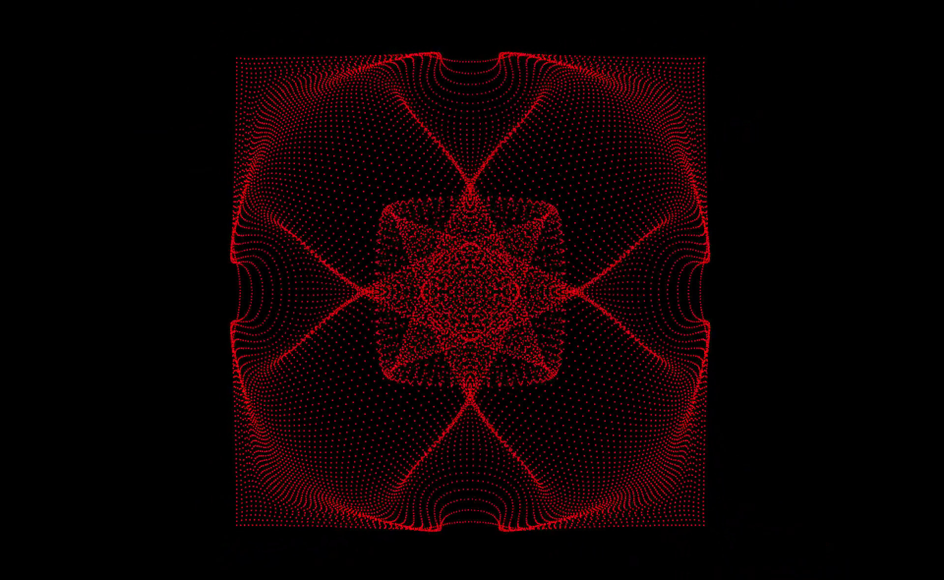
This more abstract visualization embedded in its moving glory at the start of this article was generated in the same way by simply spatially shifting the fluid cells by their heavily amplified velocities instead of only coloring them.

Reaching down from the heavens

As we are displaying a simulated universe for pure entertainment purposes we have some leeway in what laws we enforce. So while in practical simulations we would have to carefully handle any external influences to enforce e.g. mass preservation, on our playground nobody prevents us from simply dumping energy into the system at the literal twitch of a finger:

Even though this interactive sandfluidbox is as simple as it gets everyone who has ever played around with falling sand games in the vein of powder toy will know how fun such contained physical models can be. Starting from the LBM code developed during this article it is but a small step to add mouse-based interaction. In fact the most complex step is transforming the on-screen mouse coordinates into lattice space to identify the nodes where density has to be added during collision equilibration. The actual external intervention into our lattice state is trivial:

float getExternalPressureInflux(uint x, uint y) {
    if ( mouseState == 1 && norm(vec2(x,y) - mousePos) < 4 ) {
        return 1.5;
    } else {
        return 0.0;
    }
}

/* [...] */

void main() {
    const uint x = gl_GlobalInvocationID.x;
    const uint y = gl_GlobalInvocationID.y;

    const float d = max(getExternalPressureInflux(x,y), density(x,y));
    const vec2  v = velocity(x,y,d);

    setFluid(x,y,v,d);

    for ( int i = -1; i <= 1; ++i ) {
        for ( int j = -1; j <= 1; ++j ) {
            set(
                x,y,i,j,
                get(x,y,i,j) + omega * (equilibrium(d,v,i,j) - get(x,y,i,j))
            );
        }
    }
}

Conclusion

As usual the full project summarized in this article is available on cgit. Lattice Boltzmann Methods are a very interesting approach to modelling fluids on a computer and I hope that the initial theory-heavy section did not completely hide how compact the actual implementation is compared to the generated results. Especially if one doesn’t care for accuracy compared to reality it is very easy to write basic LBM codes and play around in the supremely entertaining field of computational fluid dynamics. Should you be looking for a more serious framework that is actually usable for productive simulations do not hesitate to check out OpenLB, Palabos or waLBerla.